Solution of 1-Dimensional Steady State Heat
Conduction Problem by Finite Difference Method
and Resistance Formula
Mr. Madivalappa H1 , Mr. Ravindra Hawaldar2, Mr. Vasimakram Khatib3, Mr. Faizan Shaikh4, Mr. Shashank Divgi5 1, 2, 3, 4, 5
UG Mechanical Engineering Student, Girijabai Sail Institute of Technology, Karwar, Karnataka, India 3
Assistant Professor, Mechanical Engineering Dept, Girijabai Sail Institute of Technology, Karwar, Karnataka, India
Abstract: Finite Difference Method is a numerical method which is used to solve the engineering problems. Finite Difference Method is mainly preferred because of we can solve the problems which are difficult to solve from conventional engineering methods.
In this paper we are solving the one dimensional steady state heat conduction problems by finite difference method and comparing the results with exact solutions obtained by using Resistance formula. In this paper we are solving the problems by using the Resistance formula because it gives the exact solutions.
To solve the problem by Finite Difference Method we are using some mathematical applications they are Taylor series, Fourier series, crammer’s rule. After the solutions are obtained from the both methods we have to draw the graphs to show that both the obtained results are equal.
Keywords: Finite Difference Method, Resistance formula, Fourier series, Taylor series, crammer’s rule.
I. INTRODUCTION
In this paper we are solving the heat transfer problems by using the finite difference method. Same problem also solved by using the resistance formula. Because solving the problems by using resistance formula is simple and it gives the exact solutions. After this we are comparing results obtained by these two methods.
The equation for solution of finite difference method is basically obtained by 3-Dimensional general heat conduction equation, since we are solving only 1-Dimensional heat conduction problem the equation is reduced only x-direction and we are making assumption that heat generation in y and z is negligible.
Once the solution is obtained by this method we are comparing these results with the results obtained by solutions of resistance formula by assuming the area as unity (i.e. 1m2).
The general heat conduction equation in 3- Dimensional Cartesian co-ordinates given by
+ + + =
From using this equation we derived the equation for
A. Dimensional steady state heat conduction equation. For that we are assuming that temperature varying along the y and z directions is negligible.
= 0
This equation is called as partial differential equation this can simplified as given below
= 0
This equation is called as the ordinary differential equation
In the Resistance formula we are using Fourier’s law of heat conduction equation and thermal resistance Fourier’s law of heat conduction equation is given below
II. METHODS AND METEDOLOGY
In this paper we are solving the 1-Dimensional steady heat conduction problems by using two different methods they listed below:
1) Finite Difference Method
2) Resistance Formula
A. Finite Difference Method
Finite difference method is one of the major problem Solving tool in the Engineering applications. The problems which cannot solve by analytical method that kind of problems can solve by using Finite Difference Method. For example we have solved one problem using Finite Difference Method as below:
Consider a copper rod which having a length 1m and the initial temperature at the node 1000cand the final node temperature is 10000
Fig 1 One Dimensional copper rod.
For copper we know that: K = 400W/mk0
=
Cp= J/kg k
Heat conduction problem can be solved by the general Heat Conduction equation in 3- Dimensional co-ordinate is
+ + + = (1)
Where,
T = T(x, y, z, t);
x, y, z spatial co-ordinates
α= thermal diffusivity ( )
α= k/ρC
K = thermal conductivity W/mk
ρ= density kg/
C = specific heat capacity J/kgk
g = volumetric rate of internal heat generation
Assumption of material conductivity
kx, ky, kz which are change along x, y, z axis (homogeneous)
kx = ky, = kz = k (isentropic)
The equation (1) is reducing to simpler form for the steady state heat conduction with no heat generation.
In the 1 – Dimensional problem the temperature is not much changing the parameter in y and z directions comparing with x- direction
For no heat generation g = 0
The temperature in the rod is not dependent of its time means it is a steady state one
The above equation is in the form of differential one we need to convert it into ordinary differential equations
= 0 (3)
Where T = T(x)
Equation (3) is having second ordinary differential equation includes constant co-efficient and it can be solved easily. So further it we can have to integrate the equation with respect to x and we get
= A (4)
Now we have one constant integration, for two it need to integrate again
T = Ax + B (5) Where A and B are the constant of integration
Now we have two constant of integration than we can use it in Boundary condition problems so the value to be applied in the equation (5).
At x = 0 T = Tend1 = 100℃
At x = 1m T = Tend2 = 1000℃
By substituting these Boundary values in equation (5), we get:
100 = A (0) + B B = 0
1000 = A (1) + B 1000 = A + 100 A = 900
Here the equation (5) becomes
T(x) = 900x + 100 (6)
Here we are using finite difference method for solving the above equation
Here we are using Taylor series of expansion of continuous function. The brief information about the Taylor series is explained below:
f(x+∆x) = f(x) + f1(x) ∆x + f11(x) ∆x2/2! (7) This is called as forward Taylor series expansion
f (x-∆x) = f(x) – f1(x) ∆x + f11(x) ∆x2/2! (8)
Here ∆x is very small value and ∆x2 is even smaller so we neglected these values On adding the equations (7) and (8) and truncating after the second derivative we get f(x + ∆x) + f(x -∆X) = 2 f(x) + f11(x) + f11(x) ∆x2
f11(x) = (f(x-∆x)-2 f(x) + f(x + ∆x)) /∆x2 (9)
This obtained equation is called as centered difference approximation. From the equation (3) which is also called as governing equation. T11(x) = 0; T = T(x)
T(x=0) = Tend1;
T(x=L) = Tend2 (10)
By using FDA, we are replacing second order derivative with it we get,
T −2T + T
∆x = 0
Tm-1 – 2 Tm +Tm+1 = 0 (11)
The above equation is called as FDA of original equation In this equation the m is indicates location of nodes
In the given problem we know the temperature of node 1 and node 6
We have to consider node 2 to 5 which are called as interior nodes for applying the equation (11) Let m= 2 the equation (11) becomes
T1- 2T2 + T3 = 0
Similarly for the other nodes m = 3, 4, 5 we get
T2 – 2 T3 + T4 = 0
T4 – 2 T5+ T6 = 0
Here we know the temperature of T1 and T6 they moved to RHS. So we rearranging the above equations they are given below
-2T2 + T3 = -T1
T2 – 2T3 + T4 = 0
T3 – 2T4 + T5 = 0
T4 – 2T5 = -T6
These above equations can be writing in terms of matrix form as below:
2
1
0
0
1
2
1
0
0
1
2
1
0
0
1
2
5 4 3 2T
T
T
T
=
1000
0
0
100
The various methods can be apply to solve the above equations they are give as below: Thomas algorithm method
Gauss- seidel method
Successive over relaxation (SOR) and crammer
By using the Crammers method we solve these equations as given below:
-2T2 + T3 = -100
T2- 2T3 + T4= 0
T2- 2T3 + T4 = 0
T3- 2T4 = -1000
D = 2 1 0 0 1 2 1 0 0 1 2 1 0 0 1 2
D = 5
D1 =
2 1 0 1000 1 2 1 0 0 1 2 0 0 0 1 100
D1 = 1400
D2 =
2 1 1000 0 1 2 0 0 0 1 0 1 0 0 100 2
D2 = 2300
D3 =
2 1000 0 0 1 0 1 0 0 0 2 1 0 100 1 2
D4 =
1000 1
0 0
0 2 1 0
0 1
2 1
100 0
1 2
D4 = 4100
So the final values of temperature with respect their nodes as written below:
T2 = = =280℃
T3 = = = 460℃
T4 = = =640℃
T5 = = =820℃
B. By Using Heat Resistance Formula
In this method we are using Fourier’s law of heat conduction equation and thermal resistance to solve this one dimensional copper rod.
1) Fourier’s laws of heat conduction: This law states “ The rate of flow of heat through a simple homogeneous solid is directly proportional to the area of the section at right angles to the direction of heat flow, and to change of temperature with respect to the length of the heat flow”.
The expression is given below:
Q∝
Where,
Q = Heat flow through a body per unit time (in watts), W A = Surface area of heat flow, m2
dt = Temperature difference of the faces of block
thickness ‘dx’ through which heat flows, 0C or K , and dx = thickness of body in the direction of flow, m
Thus,
Q = -k .A
Where,
k = constant of proportionality and is known as thermal conductivity of the body.
The negative sign of k shows the decreasing temperature along with the direction of where increasing thickness.
2) Thermal Resistance (Rth): The two physical systems can be prescribe by similar equation and also boundary conditions, can be called analogous. Comparison of heat transfer process has been done with flow of electricity in electrical resistance. The electrical resistance is directly proportional to potential difference by the flow of electric current. Following this also heat flow rate (Q) is directly proportional to temperature variation. The driving force is use as medium of heat conduction.
According to ohm’s law,
Current (I) = ( )
( ) (12)
By the Fourier equation, heat floe equation can be written as:
Heat flow rate (Q) = ( ) (13)
Comparing between equations (12) and (13), we get Thermal conduction resistance (Rth)cond.
Fig 3 Thermal resistance through a body.
Similarly,
R1 = R2 = R3 = R4 = R5 = 10-4
We know that,
Q =
Q =
× ×
Q = 360000w = 360kw
Q =
Q = 360 × 103 =
×
T2 = 2800C
Q =
Q = 360 × 103 =
×
T3 = 4600C
Q =
Q = 360 × 103 =
×
T4 = 6400C
Q =
Q = 360 × 103 =
×
T5 = 8200C
III. RESULTS AND DISCUSSION
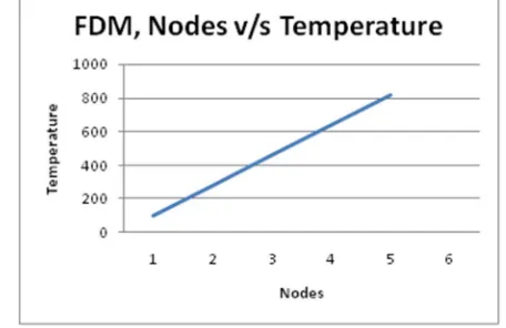
The results which are obtained by the finite difference method, the temperature at the each node as listed below in the table: List of temperatures with respect to their nodes which are obtained by Finite Difference Method, are listed below,
TABLE 1
Node Temperature
1 100
2 280
3 460
4 640
5 820
The graph of nodes v/s temperature for the above values plotted below
Graph of Temperature v/s nodes, x-axis; nodes y- axis; temperature
[image:7.612.189.417.94.242.2]In the above graph shows the results obtained by the Finite Difference Method. In the above graph the horizontal axis (x-axis) represents the node in the same the vertical axis (y-axis) represents he temperature. In the graph we come to know that the temperature goes on increasing due to because of in the rod the temperature at the initial boundary maintained at 1000c and other end at 10000c.
TABLE 2
List of results obtained by the resistance formula; Node Temperature
1 100 2 280 3 460 4 640 5 820 6 1000
The graph of nodes v/s temperature for the above values as plotted below,
Graph of nodes v/s temperature for resistance formula
In the above graph it shows that the values of the temperature obtained by using resistance formula. In the graph the horizontal axis (x – axis) shows the values of nodes and vertical axis denotes the values of the temperature.
IV. CONCLUSION
REFERENCES
[1] Mehran Makhtoumi, Dept. of Aerospace Engineering Science and Research Branch, IAU Tehran, Iron, “Numerical Solution of Heat Diffusion Equation Over One Dimensional Rod Region” vol.7 No3 May 2017,ISSN 2221-8386.
[2] Young Min Han, Joo Suk Cho and Hyung Suk Kang, “Analysis of a One-Dimensional Fin Using The Analytic Method and the Finite Difference Method” vol.9 No.1 91-98, 2005.
[3] Er.R.K.Rajput “Heat and Mass Transfer” fifth Edition 2012.