Manuscript received December 08, 2011. This research is sponsored in part by the Danish Maritime Fund under the BAYSTOW project.
or at the side (e.g., a yacht) and non-containerized break-bulk like windmill wings.
Hatch cover Bay
Line of sight
[image:2.595.46.291.92.150.2]Lashing bridge
Fig. 2. The arrangement of bays in a small container vessel.
The cargo space of a vessel is composed of a number of bays, which are a collection of container stacks along the length of the ship. Each bay is divided into an on-deckand below-deckpart by ahatch cover, which is a flat water tight structure that prevents the vessel from taking in water. An overview of a vessel layout is shown in Figure 2.
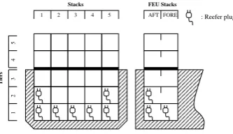
Figure 3 shows how each stack is composed of two Twenty foot Equivalent Unit (TEU) stacks and one Forty foot Equivalent Unit (FEU) stack, which hold vertically arranged cells indexed by tiers. The TEU stack cells are composed of twoslots, which are the physical positioning of a 20-foot container. The aftslot refer to the position toward the stern of the vessel, whileforeslots are allocated on the bow side. Some of the cells have access to power plugs.
The loading and unloading of containers are carried out byquay cranesthat can access the stacks individually. Some cranes can lift two 20-foot containers at the same time, but they only have access to the container on top of the stack.
: Reefer plug AFT FORE
FEU Stacks
1 2 3 4 5
1
5
4
2
3
Stacks
[image:2.595.85.252.401.497.2]Tiers
Fig. 3. A bay structure seen from behind (left) and from the side (right).
The primary objective of stowage planning is to minimize port stay. An important secondary objective is to generate stowage plans that are robust to changes in the cargo forecast. The reason is that the number of containers of each type to load in downstream ports is only fairly accurately known a few ports ahead.
When a set of containers to stow in a bay has been decided, the positioning of these containers has limited interference with containers in other bays. For this reason, it is natural to divide the constraints and objectives of the stowage planning problem into high-level inter bay constraints and objectives and low-level intra bay constraints and objectives.
High-level constraints mainly consider the stability of the vessel as defined by its trim, metacentric height, and stress moments such as shear, bending and torsion. In addition, any distribution of containers to bays must satisfy weight and volume capacity limits as well as capacity limits of the different container types. High-level objectives include the minimization of the crane makespan and of the overstowage between on and below deck.
Since we focus on slot planning in this paper, we describe the low-level constraint and obecjtives in more detail.
Low-level constraints are mainly stacking rules. Containers must be stowed forming stacks, taking into consideration that two 20-foot containers cannot be stowed on top of a 40-foot container (this is due to the lack of supports in the middle of a 40-foot container). Each stack has a maximum allowed height and weight which cannot be exceeded. Each cell can have restrictions to which kind of containers it can hold. Some cells can be, for example, reserved to only 40-foot containers. Reefer containers require power, and can only be stowed in cells with access to special power plugs. Dangerous goods (IMO containers) must be stowed following predefined security patterns, while OOG containers can only be stowed where sufficient space is available. On-deck special rules also apply due to the use of lashing rods. On deck container weight must decrease with stack height. Wind also imposes special stacking patterns on deck and line of sight rules restrict the stack heights.
Low-level objectives reflect rules of thumb from stowage coordinators in order to get stowage plans that are robust to changes in forecasted demands. The objectives include maximizing the number of empty stacks, clustering of con-tainer’s discharge port in stacks, minimizing the number of reefer slots used for non-reefer containers, and minimizing overstowage between containers in the same stack.
Taking all industrial constraints and objectives into account is desirable, however, it makes an academic study of the problem impractical. to that end, we have together with our industrial partner defined a representative problem where the number of constraints and objectives is reduced but the structural complexity is kept.
Here we give a formal definition of this representative problem using the IP model given in [2]. Given a set of stacks Sand the sets of tiers per stacksTsof the bay section for slot planning, we indicate a cell by a pair of indexess∈S and t∈Ts. Letxstc ∈ {0,1}be a decision variable indicating if the cells indexed bys∈S andt∈T contains the container c∈C, whereC is the set of all containers to be stowed in the bay section.
1 2
X
c∈C20
xs(t−1)c+ X
c∈C40
xs(t−1)c− X
c∈C40
xstc ≥0
∀s∈S, t∈Ts (1)
X
c∈C20
xs(t−1)c+ X
c∈C40
xstc≤1 ∀s∈S, t∈Ts (2)
1 2
X
c∈C20
xstc+ X c∈C40
xstc≤1 ∀s∈S, t∈Ts (3)
xstc = 1 ∀(s, t, c)∈P (4)
X
s∈S X
t∈T
xstc= 1 ∀c∈C (5)
X
c0∈C20
xstc0−2xstc ≥0 ∀s∈S, t∈Ts, c∈C20 (6)
X
c∈C
Rcxstc− Rst ≤0 ∀s∈S, t∈Ts (7)
X
t∈Ts
X
c∈C
Wcxstc≤ Ws ∀s∈S (8)
X
t∈Ts
1
2 X
c∈C20
Hcxstc+X c∈C40
t−1 X
t0=1
d−1 X
d0=2 X
c∈C
Acd0xst0c−2(t−1)δstd≤0
∀s∈S, t∈Ts, d∈D
(10)
Acdxstc+δstd−oc≤1 ∀s∈S, t∈Ts, c∈C (11)
es−xstc ≥0 ∀s∈S, t∈Ts, c∈C (12)
psd−Acdxstc≥0 ∀s∈S, t∈T, d∈D, c∈C (13)
Constraints (1) and (2), whereC20⊆CandC40⊆C are respectively the set of 20-foot and 40-foot containers, forces containers to form valid stacks where 20-foot containers cannot be stowed on top of 40-foot onces. Constraint (3) ensures that either 20-foot or 40-foot containers can be stowed in a cell but not both at the same time. The set P of containers already onboard is composed of triples(s, t, c) indicating that container c ∈ C is stowed in stack s ∈ S and tier t ∈ Ts. Constraint (4) forces those containers to their preassigned cell. Cells holding 20-foot containers must be synchronized, meaning that they cannot hold only one 20-foot container. Such contraint is handled by inequality (6). Constraint (7), whereRc ∈ {0,1} indicates if container c∈Cis a reefer container andRstholds the reefer capacity of a cell, enforces the reefer cells capacity. GivenWc as the weight of container c∈ C, constraint (8) limits the weight of a stack s ∈ S to not exceed the maximum weight Ws. Similarly the height limit is enforced by constraint (9), where Hc indicates the height of container c ∈ C and Hs is the maximum height of stacks∈S. Constraint (10) defines the indicator variable δstd which indicates if a container below the cell in s∈S and t∈Ts is to be unloaded before port d∈D, whereD is the set of discharge ports. The constant Acd∈ {0,1}indicates if containerc∈Cmust be discharged at portd∈D. Constraint (11) then uses theδstd variable to count overstowage into the variableoc. The number of non-empty stacks is stored in the variable es via the constraint (12). The number of discharge ports used within a stack is then calculated into the variablepsd in constraint (13).
An optimal solution to slot planning minimizes the fol-lowing objective:
100X c∈C
oc+ 20X s∈S
X
d∈D
psd+ 10X s∈S
es+
5X s∈S
X
t∈Ts
Rst
X
c∈C40
xstc(1−Rc)+X c∈C20
xstc(1
2Rst−Rc) (14)
which, following the priorities of the stowage coordinators, minimizes: overstowage, the number of different discharge ports in a stack, the number of non-empty stacks and the number of reefer cells used by non-reefer container.
III. LITERATURESURVEY
The number of publications on stowage planning has grown substantially within the last few years. Contributions can be divided into two main categories: single-phase and multi-phase approaches. Multi-phase approaches decompose the problem hierarchically. 2-phase [4], [5], [6], [1] and 3-phase approaches [7], [8] are currently the most successful in terms of model accuracy and scalability. Single-phase approaches represent the stowage planning problem (or parts of it) in a single optimization model. Approaches applied include IP [9], [10], [11], [12], CP [13], [3], GA [14],
[15], SA [16], placement heuristics [17], 3D-packing [18], simulation [19] , and case-based methods [20].
Slot planning models and algorithms in the work above, however, either do not solve sufficiently representative ver-sions of the problem or lack experimental evaluation. In our previous work, we have used the same representative model as in this paper. In [3] and [2] a CP approach is used to solve this model. The CP model solved with Gecode [21] was shown to greatly outperform both the IP model given in this paper solved with CPLEX and a column generation approach. As our comparison with the CP approach in this paper shows, however, these exact methods may need long time to prove optimality.
IV. SOLUTIONAPPROACH
As mentioned in Section I, the aim of slot planning is to stow containers within a bay section (also called a location) as fast as possible. Knowing that up to 100 slot planning instances must be solved for a stowage plan and that master planning is time consuming, it easy to argue that a 1 second time limit on slot planning is adequate.
In order to reach or even improve such high performance we propose a CBLS with a simple hill-climbing search. Details about CBLS can be found in [22], however, some of the basic principles can easily be captured by the following description of the algorithm used in this work.
Hill-climbing might seem like a simplistic approach espe-cially when the objectives of the problem are clearly non-linear. Our choice for this search method is supported by the fact that fast solutions must be found. We concentrated our effort on developing an accurate guiding heuristic, which, in combination with incremental computations is able to drive the hill-climb towards (near-)optimal solutions. The search could be probably be improved using a metaheuristic framework. Our preliminary studies, however, show that this is non-trivial due to the structure of the problem.
We model slot planning with a set of decision variables xstp ∈C∪{⊥}defining which container is to be stowed into which slot (one cells is composed of an AFT and a FORE slot). Slots are identified by a triple(s, t, p)wheres∈S is the stack,t∈Tsis the tier andp∈P ={AF T, F ORE}is the position within the cell. Slots without stowed containers are assigned the special value ⊥. Unlike the original IP model, which was cells based, our CBLS model is slot based. Such a model is more robust in terms of future development when slot based constraints need to be applied.
The algorithm uses a neighborhood generated by swapping containers. A swap is an exchange of some containers between a pair of cells. Formally, a swap γ is a pair of tuples γ = (hs, t, ci,hs0, t0, c0i) where the containers c in
the cell at stack s and tier t exchange position with the containersc0in the cell at stacks0and tiert0. The setscandc0 can contain at most two containers. Swaps are implemented with two functions swap20 for exchanging position of 20-foot containers ( that is one 20-20-foot with another or with an⊥container), andswap40 for exchanging position of 40-foot containers (with an other 40-40-foot, or with a mixture of 20-foot and⊥containers).
consideration. Once a constraint has no violation it is con-sidered satisfied, thus a solution where all constraint have no violation is a feasible solution. Given an assignment π, let xπ
stp be the value of the decision variables for assignment π. Taking constraint (1) as an example the violations for a single slot can be defined as
vstpπ = t−1 X
t0=0
¬(t(xπstp =⇒ ¬f(xπst0AF T)) (15)
wheret(c)is true ifc∈Cis a 20-foor container,f(c)is true if c ∈ C is a 40-foot container. We also represent boolean variables as{0,1}and allow arithmetic operations over them. The total violation for constraint (1) is thus defined as
X
s∈S X
t∈T X
p∈P
vstpπ (16)
Violations are also used during the search as heuristic guid-ance, as it will soon be described in the description of the search algorithm.
Objectives are defined, in terms of violations like the constraints. A solution minimizing the objective violations is optimizing the objective. Violations for the overstowage objective (11) are, for example defined for each slot as
oπstp=∃t0∈ {0, ..., t−1}, p0∈P.
dsp(xπstp)> dsp(x π
st0p0) (17)
wheredsp(c)indicates the discharge port of containerc. The total numer of overstowing containers thus is
X
s∈S X
t∈T X
p∈P
oπstp (18)
Other constraints and objectives are defined in a similar fashion. A comprehensive definition is found in [23].
A. A 3-Phase approach
Constraint satisfaction and objective optimization, tend to drive the search in opposite directions, ultimately generating a poor heuristic. For this reason we decided to split the main search into a feasibility and optimality phase. We start with a greedy initial solution, generated by relaxing the stack height and weight constraint. Containers are then stowed using the lexicographical order (reefers≺discharge port≺
20-foot container), designed to optimize the objective func-tion. Containers that cannot be stowed, due to the constraints, are then sequentially stowed at the end of the procedure. This, placement heuristic, produces high quality solution that are slightly infeasible. Such solutions become the in-put of the feasibility phase where only the violation of the constraints are minimized. Feasible solutions are then passed to theoptimality phasewhich will now only consider feasible neighborhoods and optimize the objective functions. Both the feasibility and optimality phases use a min/max heuristic where swaps are chosen by selecting a slot with the maximum number of violations and swapping it with a slots producing the minimum violations ( in other words, the most improving swap). This is how violations become the essential building blocks of the search heuristic.
Algorithm 1 shows the details of the search. The placement heuristic is used in line 1 to generate and initial solutionπ. Lines 2-6 are the implementation of the feasibility phase.
Algorithm 1: SolveLocation()
π=placementHeuristic(); /* Heuristic Placement 1
*/
while¬satisfy(constraints)do 2
π0←π; /* Feasibility phase */
3
selects1←most violated slotdo
4
selects2←most improving slot to swapdo
5
π←swap(s1, s2);
6
ifπ0=πthen perform side move
7
whilethere is objective improvementdo
8
π0←π; /* Optimality phase */
9
selects1←most objective violating slotdo
10
selects2←most objective improving feasible slot to
11
swapdo
π←swap(s1, s2);
12
ifπ0=πthenπ=perform tie-breaking swap onπ 13
returnπ; 14
While the constraints are not satisfied (line 2), we perform swaps (line 6) selecting the most violated slot (line 4) and the most improving slot (line 5). If the swap generates a non improving (but not worse) solution, we accept the solution as a side move. Side moves are allowed only after a number of failed improving tentatives.
Lines 8-13 are the implementation of the optimality phase. With π now being a feasible solution, we perform feasible swaps (line 12) so long as an objective improvement can be generated. Similarly to the feasibility phase, lines 10-11 select the most violating and most improving slots. The selection, however, is limited to feasible swaps (swaps that do not generate any violations on the constrains). Should the swap generate a non-improving solution, a limited number of side moves are allowed where solutions are chosen using tie-breaking rules (line 13). For the overstowage objective (11) the tie-breaking is defined as the number of containers overstowed by each container, which will make the algorithm choose a container that overstows many containers over one that only overstows a single container. For the non-empty stack objective (12) the tie is broken by the number of containers in the stack, so that the search rather swaps containers that are in almost empty stacks. The clustering objective (13) calculates the tie-breaker by summing the quadratic product of the number of containers with the same discharge port, which will favor those stacks that have the most containers with the same discharge port.
B. Incremental computations
In order to efficiently compute and evaluate the neigh-borhoods, we designed incremental calculations for each constraint and objective. Incremental calculations (or delta evaluations) allow the algorithm to evaluate and apply swaps efficiently without having to recompute all of the constraint and objective violations. A delta evaluation is based on a simple construction/destruction principle, where the viola-tions of the original assignment are first removed from the total violation, to then be reinserted according to the new assignment. A delta evaluation can be made volatile, thus only be used as an evaluation, or persistent if the change has to be applied to the solution.
TABLE I
Test Set Characteristics. THE FIRST COLUMN IS AN INSTANCE CLASSID. COLUMN2, 3, 4,AND5INDICATE WHETHER40-FOOT, 20-FOOT, REEFER,AND HIGH-CUBE CONTAINERS ARE PRESENT. COLUMN6 INDICATES WHETHER MORE THAN ONE DISCHARGE PORT IS PRESENT.
FINALLY,COLUMN7IS THE NUMBER OF INSTANCES OF THE CLASS.
Class 40’ 20’ Reefer HC DSP>1 Inst.
1 √ 6
2 √ 18
3 √ √ 4
4 √ √ 42
5 √ √ √ 27
6 √ √ √ 8
7 √ √ √ √ 7
8 √ √ √ 7
9 √ √ √ √ 10
10 √ √ √ √ 2
11 √ √ √ √ √ 2
containerc. Then we look at all the containers stowed above it, removing one violations for each of the ones that only overstow container c. Now all the violations connected to container c are removed. Swapping c withc0 we now have to do a similar but opposite operation where we add 1 violation to all container that only overstow c0 in stack s at tier t and 1 violation if c0 is overstowing any container
below it. The same operation is then performed on the other stack s0 where c and c0 exchange roles. It is easy to show that given the correct data structures such operations can be performed linearly with the size of the tiers under consideration. More details and formal definitions for all constraints and objectives as well as incremental evaluations can be found in [23].
V. COMPUTATIONALRESULTS
The algorithm has been implemented in C++ and all experiments have been conducted on a Linux system with 8 Gb RAM and 2 Opteron Quad Core CPUs, each running on 1.7 GHz and having 2Mb of cache. The slot planning instances have been derived from real stowage plans used by our industrial collaborator for deep-sea vessels.We use test data set of 133 instances, including locations between 6 TEUs and 220 TEUs. Table I gives a summarized overview of these instances. Notice that many instances only have 1 discharge port, this is a feature of the instances generated after a multi-port master planning phase, thus it reflects the actual problem we are facing.
The experimental results on the test data set, shown in Table II(a), show the percentage of solutions solved within a specific optimality gap (optimal solutions have been gener-ated using the constraint programming algorithm described in [2]). It is easy to see that only few instances diverge from near optimality and that in 86% of the cases the algorithm actually reached the optimal solution. Studying the algorithm performance closer, we were able to gain some insight on the quality of the different phases. The heuristic placement does not take the height and weight constraint into account, leaving space for improvements. However Table II (c) and (d) show that the solution found by the heuristic placement is not far from being feasible in most of the cases. This is supported by the fact that often feasibility is reached within 20 iterations and that 61% of the time, the objective value is not compromised. The quality of the objective value of the first feasible solution is also optimal in 74% of the
TABLE II
Algorithm Analysis(A) COST GAP BETWEEN RETURNED SOLUTION AND OPTIMAL SOLUTION. (B) COST GAP BETWEEN FIRST FEASIBLE SOLUTION AND OPTIMAL SOLUTION. (C) NUMBER OF ITERATIONS NEEDED TO FIND THE FIRST FEASIBLE SOLUTION. (D) WORSENING OF THE COST OF THE HEURISTIC PLACEMENT WHEN SEARCHING FOR THE
FIRST FEASIBLE SOLUTION.
Opt. Gap Opt. Gap (Feas.) Feas. Iter. Feas. Worse
Gap. Freq. Gap. Freq. It.≤ % Obj % %
0% 86% 0% 74% 0 29% -20% 2%
1% 2% 5% 6% 5 23% -10% 2%
2% 2% 10% 2% 10 18% -5% 4%
3% 2% 15% 5% 15 8% 0% 61%
4% 1% 20% 3% 20 6% 5% 8%
10% 1% 25% 3% 25 3% 10% 2%
15% 4% 35% 3% 30 6% 20% 7%
20% 1% 40% 1% 35 1% >20% 15%
30% 2% >100% 3% 40 2%
45 2%
50 1%
65 2%
(a) (b) (c) (d)
cases (Table II(b)), suggesting that the heuristic placement procedure is performing well. The results also point to the fact that the optimality phase improves only a limited number of instances, which however is important especially in the cases where the optimality gap after the feasibility phase is more than 20%.
The limited improvement of solutions in the optimality phase probably happens because the search does not allow for a large degree of diversification. Preliminary tests using tabu search have shown that local diversification often was unsuccessful to escape a local minimum due to large struc-tural differences between the local minimum and an optimal solution. A possible approach to solve this problem could be to less closely follow the heuristic in the initial placement and the search procedures. This method, however, would probably be more expensive in terms of runtime performance.
0 0.1 0.2 0.3 0.4 0.5 0.6 0.7
0 50 100 150 200 250
Time (sec.)
TEUs Runtime performance
[image:5.595.312.542.486.648.2]Runtime
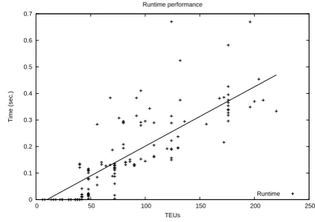
Fig. 4. Execution time as a function of instance size measured in TEUs.
0 0.2 0.4 0.6 0.8 1
0 0.2 0.4 0.6 0.8 1
CP time
LS time LS vs CP runtime comparison
[image:6.595.61.283.57.217.2]Normal Unsolved More than 5 sec. More than 3 sec.
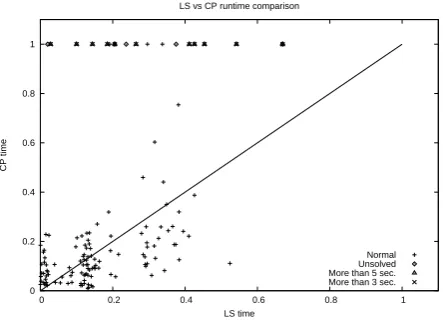
Fig. 5. Execution time comparison between our algorithm and the complete constraint programming approach used to generate optimal solutions.
were not solvable by the CP approach within 160 seconds. However, in a comparison between the two approaches these instances are particularly interesting.
As depicted, the CP approach is highly competitive within the set of instances that it can solve in 160 seconds. However our approach can solve the problematic instances for CP fast as well. This result indicates that the under-constrained nature of the problem might force exact methods to spend an excessive amount of time proving optimality. A pragmatic solution would be to execute the two approaches in parallel and rely on the optimal CP solution for the locations where it can be generated fast.
VI. CONCLUSION
We have developed an accurate slot planning model to-gether with a major liner shipping company and implemented a constraint-based local search algorithm to solve them. Our experimental results show that these problems in practice are easy even though the general problem is NP-Complete. Our work contributes to our current understanding of stowage planning. It shows that if these problems are combinatorially hard in practice, the main challenge is to distribute containers to locations in vessel bays rather than assigning them to individual slots in these bays.
REFERENCES
[1] D. Pacino, A. Delgado, R. M. Jensen, and T. Bebbington, “Fast generation of near-optimal plans for eco-efficient stowage of large container vessels,” inICCL, 2011, pp. 286–301.
[2] A. Delgado, R. M. Jensen, K. Janstrup, T. H. Rose, and K. H. Andersen, “A constraint programming model for fast optimal stowage of container vessel bays,”European Journal of Operations Research, 2011, [Accepted for publication].
[3] A. Delgado, R. M. Jensen, and C. Schulte, “Generating optimal stowage plans for container vessel bays,” inProceedings of the 15th Int. Conf. on Principles and Practice of Constraint Programming (CP-09), ser. LNCS Series, vol. 5732, 2009, pp. 6–20.
[4] I. D. Wilson and R. P., “Principles of combinatorial optimization applied to container-ship stowage planning,” Journal of Heuristics, no. 5, pp. 403–418, 1999.
[5] J. Kang and Y. Kim, “Stowage planning in maritime container trans-portation,”Journal of the Operations Research Society, vol. 53, no. 4, pp. 415–426, 2002.
[6] W.-Y. Zhang, Y. Lin, and Z.-S. Ji, “Model and algorithm for container ship stowage planning based on bin-packing problem,”Journal of Marine Science and Application, vol. 4, no. 3, 2005.
[7] D. Ambrosino, D. Anghinolfi, M. Paolucci, and A. Sciomachen, “An experimental comparison of different heuristics for the master bay plan problem,” inProceedings of the 9th Int. Symposium on Experimental Algorithms, 2010, pp. 314–325.
[8] M. Yoke, H. Low, X. Xiao, F. Liu, S. Y. Huang, W. J. Hsu, and Z. Li, “An automated stowage planning system for large containerships,” in In Proceedings of the 4th Virtual Int. Conference on Intelligent Production Machines and Systems, 2009.
[9] R. Botter and M. A. Brinati, “Stowage container planning: A model for getting an optimal solution,” inProceedings of the 7th Int. Conf. on Computer Applications in the Automation of Shipyard Operation and Ship Design, 1992, pp. 217–229.
[10] D. Ambrosino and A. Sciomachen, “Impact of yard organization on the master bay planning problem,”Maritime Economics and Logistics, no. 5, pp. 285–300, 2003.
[11] P. Giemesch and A. Jellinghaus, “Optimization models for the con-tainership stowage problem,” inProceedings of the Int. Conference of the German Operations Research Society, 2003.
[12] F. Li, C. Tian, R. Cao, and W. Ding, “An integer programming for container stowage problem,” inProceedings of the Int. Conference on Computational Science, Part I. Springer, 2008, pp. 853–862, LNCS 5101.
[13] D. Ambrosino and A. Sciomachen, “A constraint satisfaction approach for master bay plans,”Maritime Engineering and Ports, vol. 36, pp. 175–184, 1998.
[14] Y. Davidor and M. Avihail, “A method for determining a vessel stowage plan, Patent Publication WO9735266,” 1996.
[15] O. Dubrovsky and G. L. M. Penn, “A genetic algorithm with a compact solution encoding for the container ship stowage problem,” J. of Heuristics, vol. 8, pp. 585–599, 2002.
[16] M. Flor, “Heuristic algorithms for solving the container ship stowage problem,” Master’s thesis, Technion, Haifa, Isreal, 1998.
[17] M. Avriel, M. Penn, N. Shpirer, and S. Witteboon, “Stowage planning for container ships to reduce the number of shifts,”Annals of Oper. Research, vol. 76, pp. 55–71, 1998.
[18] A. Sciomachen and A. Tanfani, “The master bay plan problem: a solution method based on its connection to the three-dimensional bin packing problem,”IMA Journal of Management Mathematics, vol. 14, pp. 251–269, 2003.
[19] W. C. Aye, M. Y. H. Low, H. S. Ying, H. W. Jing, and Z. Min, “Visualization and simulation tool for automated stowage plan gener-ation system,” inProceedings of the International MultiConference of Engineers and Computer Scientists 2010 (IMECS 2010), vol. 2, Hong Kong, 2010, pp. 1013–1019.
[20] S. Nugroho, “Case-based stowage planning for container ships,” in
The Int. Logistics Congress, 2004.
[21] Gecode Team, “Gecode: Generic constraint development environ-ment,” 2006, available fromhttp://www.gecode.org. [22] L. Michel and P. V. Hentenryck, “A constraint-based architecture for
local search,”ACM SIGPLAN Notices, vol. 37, no. 11, pp. 101–110, nov 2002.