Numerical Transport Simulations in
Semiconductor Nanostructures on CPUs and GPUs
Jan Jacob, Lothar Wenzel, Darren Schmidt, Qing Ruan, Vivek Amin, and Jairo Sinova
Abstract—We present numerical simulations of charge trans-port through semiconductor nanostructures performed within the Green’s function formalism. The commonly used algorithm to compute the conductance of nanostructures in this formalism has been adapted for parallel execution on both multicore com-puters and general-purpose graphics processing units (GPU). Additionally, memory utilization has been optimized so that larger systems may be simulated, enabling realistic device sizes.
Index Terms—numerical simulation, Green’s function, GPU, multicore, algorithm.
I. INTRODUCTION
T
HE continuing miniaturization of circuits comes not without side effects; as the dimensions of such devices decrease, quantum effects become relevant to their operation. While these effects can be detrimental to standard CMOS devices, they also pave the way for new devices that have the potential for performance improvements. Spin-based tran-sistors, utilizing magnetic source and drain contacts along with a spin-orbit coupled semiconductor channel, provide an important example. Such devices would require less energy for switching processes, since their channels no longer have to be depleted completely [1]. By using gates, one can influence an electron’s spin precession length and change its spin orientation with respect to the magnetization of the drain electrode [2]. Such controllable phenomena could lead to a new spin-based information processing paradigm. Although the physics of charge-based devices is well under-stood, physicists and engineers still face challenges regarding the experimental realization of their spin-based cousins. While analytical predictions regarding these nanoscale de-vices can be made, direct comparison with experiments is challenging and often impossible due to the oversimplifi-cation of the analytical model. However, numerical trans-port simulations of nano-structured semiconductor devices provide a very important bridge between analytical descrip-tions and experimental results. Such simuladescrip-tions can account for donor impurities, lattice imperfections, and interactions within a sample that are ordinarily inaccessible to mostManuscript received December 30, 2011; revised December 30, 2011. This work was supported in part by the Deutsche Forschungsgemeinschaft via the Graduiertenkolleg 1286 ”Functional Metal-Semiconductor Hybrid Systems” and Project Me916/11-1 ”Spin-Filter Cascades in InAs Het-erostructures”, the Free and Hanseatic City of Hamburg via the Center of Excellence ”‘Nanospintronics”’, the Office of Naval Research via ONR-N00014110780, and the National Science Foundation by NSF-MRSEC DMR-0820414, NSF-DMR-1105512, NHARP
J. Jacob is with the Institute of Applied Physics, University of Hamburg, Germany, e-mail: [email protected]
L. Wenzel, D. Schmidt, and Q. Ruan are with National Instruments, Austin, TX, USA e-mail: [email protected], [email protected], [email protected]
V. Amin and J. Sinova are with the Department of Physics and As-tronomy, Texas A& M University, College Station, TX, USA, e-mail: [email protected], [email protected]
analytical computations, providing researchers with more accurate predictions to compare with experiments. Unfortu-nately, it is extremely challenging to simulate these devices with both realistic dimensions and appropriately minute grid sizes, due to the large computational and memory load. One of the common approaches to simulate transport in semiconductor nanostructures is the non-equilibrium Green’s function (NEGF) method [3]. Other popular approaches, such as the stabilized transfer matrix algorithm [4], can be translated in terms of the NEGF method; it exhibits a similar mathematical structure and thus employs complementary numerical techniques. In this work we explore optimized implementations of the Green’s function method and their scalability over multiple threads, as well as their portability to general purpose graphics processing units (GPU).
II. MATHEMATICAL AND PHYSICS BACKGROUND We briefly introduce the Green’s function method to simu-late transport in mesoscopic structures [3] whose dimensions are smaller than the coherence length. Here the conductance must be calculated by the Landauer formula, where the trans-mission probabilityT describes the transmission probability of carriers through the sample from one contact to the other. Overall the Landauer formula is given by
G=2e 2
h T (1)
whereeis the elementary charge andhis Planck’s constant. In these systems there exist different quantum-mechanical modes in which carriers can propagate through. We define the matrix elementssmn as the probability amplitudes for a carrier entering the sample in them-th mode of one contact to leave in then-th mode of the other contact.
If the conductor is much smaller than the phase-relaxation length, then transport is coherent and the total transmission probability can be decomposed into the sum of these ampli-tudes squared. Thus one may write
G= 2e 2
h X
m,n
Tmn, (2)
where,
Tmn=|smn|
2
. (3)
Thus by determining the s-matrix of the microscopic sam-ple, one can compute the conductance using the Landauer formula. Green’s functions provide a convenient way to do this. We begin by defining a Green’s function, for a system governed by some HamiltonianHˆ(r)
h
the Green’s function to simply be the wave function given in terms of the position vector r that describes the location of the source. To calculate the Green’s function the above concept is applied to a tight-binding model by the method of finite differences, such that
G(r, r0)→Gij, (5) whereiandj are indices denoting different lattice positions corresponding to r and r0. As a result the aforementioned differential equation becomes a matrix equation
[EI−H]G=I, (6)
where each row or column in the above matrices stands for a particular lattice site within the entire sample. Therefore the matrix for a two-dimensional system of Nx horizontal sites andNy vertical sites is of dimension NxNy×NxNy. Since we have converted the Hamiltonian from a differential operator to a matrix operator, we must introduce discretized derivative operators, given by
dF dx
x=(j+1 2)a
→ 1
a[Fj+1−Fj] (7) d2F
dx2
x=ja
→ 1
a2{Fj+1−2Fj+Fj−1}. (8)
As an example of a Hamiltonian matrix for a one-dimensional system, with a simple kinetic and potential term, one can consider,
H =
· · · −t 0 0 0
−t U−1+ 2t −t 0 0
0 −t U0+ 2t −t 0
0 0 −t U1+ 2t −t
0 0 0 −t · · ·
, (9)
wheret= ¯h2/2ma2 is the so-called hopping parameter and
Ui denotes the potential at each lattice site. Such a matrix can be rewritten for two or three dimensional systems given an appropriate labeling system. Written in this way, one can compute Gthrough matrix inversion.
G= [EI−H]−1. (10) It should be noted that there exist two independent solutions for G, normally referred to as the retarded and advanced Green’s functions; often an imaginary parameter is added to the energy in Eqn. 10 in order to force the solution to be one or the other. For our present purposes we shall omit this imaginary factor. As solutions like Eqn. 10 for Hamiltonians such as Eqn. 9 only provide information about scattering within a sample, the concept has to be expanded to include the leads. One normally proceeds by assuming that the sample is connected to the leads at various lattice sites, and that only the directly neighboring sites within the lead itself are relevant to compute the lead’s full effect on transmission. If the leads are semi-infinite, homogeneous, and reflection-less, one can show that this is an exact statement. We shall consider the case in which there are two leads, labeled p and qand the sample is denoted as c. Our sample shall be represented by aNx×Ny grid, where thex-direction runs horizontal and the y-direction runs vertical. Each lead shall be connected fully to either vertical side of the sample, giving
Nyneighboring points in each lead. One can then rewrite the Green’s function in block matrix form as
G=
Gc Gcp Gcq Gpc Gp 0 Gqc 0 Gq
. (11)
All carriers enter or leave the sample via Gcp or Gcq and propagate throughout the sample viaGc. Propagation within the leads themselves is included viaGp or Gq. One can see through inspection of the block matrix that there is no direct connection between differing leads; carriers must transmit through the sample to travel between p andq. We assume the following structure for G:
G=
EI−Hc τp τq τp† EI−Hp 0 τq† 0 EI−Hq
−1
. (12)
Note that each element in the above block matrix has different dimensions, depending on the number of lattice sites corresponding to the portion they describe. By assuming that a carrier may only enter the sample through a site horizontally adjacent to the lead, one may write
[τp(q)]ij =tδij. (13)
and solve forGc. One can show, after some algebra, that
Gc= [EI−Hc−Σ]−1, (14) where
Σ =
t2gp 0 0
0 0 0
0 0 0
+
0 0 0
0 0 0
0 0 t2gq
= Σp+ Σq (15)
and
gp(q)=
EI−Hp(q)
−1
(16)
TheΣp(q) areNxNy×NxNy matrices, whilegp andgq are Ny×Nymatrices. Equation 14 describes the Green’s function in terms of the hopping parameter t, the Fermi energy E, the conductor’s HamiltonianHc, and the lead’s Hamiltonians Hp(q). The transmission probability is then calculated by
T =X
m,n
Tmn=TrΓpGcΓqG†c
, (17)
where
Γp(q)=i[Σp(q)−Σ†p(q)]. (18)
III. BASIC IMPLEMENTATION
Fig. 1. Flowchart for the basic Green’s function algorithm
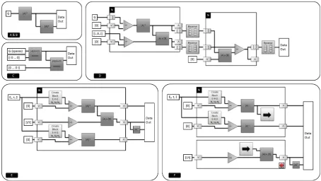
when implemented as a dense matrix. The Eigenvalue prob-lem in the second step of the size Ny ×Ny can take a significant share of computing resources for extremely large systems. The self energiesΣAandΣR are created by simple scalar operations in step three. The fourth step represents the bottleneck of this basic implementation due to the inversion of a (NxNy)×(NxNy) matrix in Eqn. 14, which will be addressed extensively below. Creating theΓmatrices in step five only involves scalar operations on the elements of ΣA andΣR and can be done in parallel to the more demanding step four. The final step six obtains the transmission and reflection coefficients from the traces given by Eqn. 17 and includes the product of four matrices of(NxNy)×(NxNy).
IV. OPTIMIZATIONS A. Analysis of the basic implementation
a) Problem 1: Memory efficiency of the matrixH: The matrixH is of the size(NxNy)×(NxNy). As it grows fast with system size this becomes the limiting memory factor. However, the structure of the matrix allows optimization of the memory performance:
HNxNy×NxNy =
. .. Y 0 0 Y X Y 0
0 Y X Y
0 0 Y . ..
, with (19)
XNy×Ny =
. .. B 0 0 B A B 0
0 B A B
0 0 B . ..
, (20)
YNy×Ny = diag[C] (21)
whereA= 4t+V(x, y),B =C=−t, with the the potential energy at a given siteV(x, y). Using the extreme sparsity of this matrix significantly enhances the memory performance. The same is true for the transverse Hamiltonian, that has an even simpler structure:
Hy=
. .. B 0 0 B D B 0
0 B D B
0 0 B . ..
, (22)
where D = 2t. However, even a sparse representation of the matrix still grows dramatically with the system size. Therefore it is most efficient to create onlyNy×Ny matrix blocks directly, when they are needed in the algorithm.
b) Problem 2: The Eigenvalue solver: The Eigenvalues of Hy represent the modes and the Eigenvector matrix yields the wave functions for the self energy matrix. While there is probably potential to optimize the algorithm for the eigenvalue solver, it is even more advantageous to com-pletely remove the numerical Eigenproblem by solving it analytically as it is a simple one-dimensional quantum well problem and the solution is known. So we do not focus on any numerical optimizations of this part.
c) Problem 3: Matrix inversion: As most of the compu-tation time is spent on the matrix inversion to determine the Green’s function in Eqn. 14 our main focus was to optimize this part. There are several ways to avoid the direct inversion of the full matrix G. One approach is to use blockwise inversion. While this improves the performance over a direct inversion and can be applied later in optimized codes to improve the performance of the remaining inversions of smaller sub-matrices, it is more advantageous to first utilize the special structure of the matrix. The optimizations are described in detail in Sec. IV-C through IV-F.
d) Problem 4: The final matrix multiplication: For Eqn. 17 eight multiplications of Ny × Ny matrices are necessary. The structure of the algorithm allows to execute four of them in parallel. The other four need the results of the first set of multiplications, but can then also be executed in parallel. By making use of high-performance matrix multiplication functions this task reaches a high level of parallel execution (see below). As the computational load of this part is small compared to the inversion no further optimizations have been done to this part.
B. First optimization: optimized linear algebra functions
National Instruments developed a LabVIEW High Perfor-mance Analysis Library (HPAL) [5]. HPAL exposes linear algebra functions from Intel’s Math Kernel Library (MKL)[6] from within LabVIEW. These functions are optimized for execution on multi-core processors and designed to work when the input matrices are extremely large.
We replace the functions for matrix multiplication and matrix inversion. The benchmark results in Section VI show that we are still limited by the inefficient use of memory by using dense matrices.
C. Second optimization: sparse matrices
To take advantage of the sparsity of the matrices, we employed the sparse matrix functions in the HPAL library replacing the inversion by the PARDISO direct sparse linear solver [7], [8]. The benchmarks show that the PARDISO solver is faster than a dense solver, but still has memory issues above Nx = Ny = 700 as the PARDISO solver generates a lot of intermediate data.
D. Third optimization: Block-Tridiagonal solver
Fig. 2. Visualization of the different algorithms for the matrix inversion
Assuming that the block tri-diagonal linear system is
A1 B1 0
C1 A2 B2
C2 A3 . ..
. .. . .. BN
x−1
0 CNx−1 ANx
X1
X2
X3
.. . XNx
=
Y1
Y2
Y3
.. . YNx
,
whereAk,Bk andCk are allNy×Ny blocks. The solution can be computed by the following two steps.
Step 1: fork from1 toNx
¯
Bk = (Ak−Ck−1B¯k−1)−1Bk
¯
Yk = (Ak−Ck−1Bk¯ −1)−1(Yk−Ck−1Yk¯ −1).
Step 2: fork fromNx to1
Xk= ¯Yk−BkXk¯ +1.
This algorithm takes advantage of the sparsity of the ma-trix to achieve significant speedup, but still requires relatively large memory. There are 3Ny Ny×Ny complex matrices generated between step 1 and step 2. ForNx=Ny= 1000, storing these matrices would need 48 GB RAM and forcing slow data exchange with hard disk media.
E. Fourth optimization: Improved Block-Tridiagonal solver
Since we only need the fourNy×Nycorners of the inverse matrix, we are solving two linear systems with the right hand sides
INy 0 . . . 0
0 ,
and
0 . . . 0 INy0 ,
where IN y is an Ny ×Ny identity matrix. We are only interested in the first and last blocks in the solutions. The
last block of each linear system is already computed after the first step in the Thomas Algorithm. Thus, we propose another method to compute the first block. Denote
K=
0 INy
INy
. ..
INy 0
.
whereK satisfies KT =K andK2=I. Furthermore, if
A=
A1 B1 0
C1 A2 B2
C2 A3 . ..
. .. . .. BN
x−1
0 CNx−1 ANx
,
then
KAK=
ANx BNx 0
CNx ANx−1 BNx−1
CN x−1 ANx−2
. .. . .. . .. B
2
0 C2 A1
.
Since(KAK)−1=KA−1K, the upper left(right) corner of
A−1 is equal to the lower right(left) corner of (KAK)−1.
The first step of Thomas algorithm withKAK would thus give the upper left(right) corner ofA−1. The new algorithm
F. Fifth optimization: Pipelined Block-Tridiagonal solver
To further improve the performance by making use of parallel architectures we pipelined sequential linear algebra calculations. By adjusting each group of operations to have roughly the same complexity, we ensured a constant high level of utilization on all available cores during the full inversion algorithm. At the same time the memory usage stays below 3 GB for system of up toNx=Ny= 1000.
V. IMPLEMENTATION ONGPUS
As the optimized pipelined block-tridiagonal solver still represents the most demanding part of our code, we further improved its performance by employing GPUs. As almost exclusively matrix multiplications and inversions have to be performed and several operations are done in parallel, GPUs yield a high performance potential. The other parts of the code focus on pre- and post-processing steps which lack computational complexity and are executed exclusively on the host processor cores. We used a prototype of the LabVIEW GPU Analysis Toolkit for the implementation on GPUs [10]. The small memory footprint of the optimized block-tridiagonal solver allows us to download the entire problem to the GPU and invoke the solver on the GPU device, retrieving only the final results. This minimizes com-munication between host and GPU during the most critical processing time. The efficient memory structure also allows the host to execute multiple independent simulation steps (i.e. as part of a sweep of e.g. potential or Fermi Energy) in parallel if more than one GPU is available.
VI. BENCHMARKS
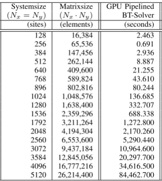
We ran code implementing the direct inversion of the Green’s function matrix (Version 0) and the different op-timizations of Sec. IV-B through IV-F (Version 1 through 5) on an IBM idataplex dx360 M3 workstation [11] with two Intel Xeon X5650 six-core processors, running at2.67 GHz, 48 GB random access memory, and two NVIDIA Tesla M2050 GPUs with 3 GB random access memory [12]. All code was written in LabVIEW 2011 using functionality provided by the High Performance Analysis Library (HPAL) and the GPU Analysis Toolkit. Internally, HPAL called Intel’s Math Kernel Library (MKL) v10.3 for execution on the CPU’s multiple cores. The GPU Analysis Toolkit invoked routines from NVIDIA’s CUDA Toolkit v4.0 and CUBLAS libraries for execution on the Tesla GPUs. The benchmarks were performed with a 64-bit version of LabVIEW 2011 running under Windows 2008 Server Enterprise Edition, with the NVIDIA Tesla GPU set to TCC mode. Results from the CPU-based implementations are shown in TABLE I. Results for the code in version 5 which executed primarily on NVIDIA’s Tesla M2050 GPUs are shown in TABLE II. The results include just the execution of the inversion algorithm described in Section IV-F. The initialization and postpro-cessing are not taken into account as they represent just a fraction of the computation time. However, the presented benchmarks include the time for transferring the data to and from the GPUs. To visualize the performance of the different implementations we summarized the results we show the number of system slices along thex-direction that can be simulated per hour on a single node or a single GPU
TABLE II
BENCHMARK RESULTS FOR THEGPUIMPLEMENTATION OF THE PIPELINED AND OPTIMIZED BLOCK-TRIDIAGONAL MATRIX INVERSION
SOLVER
Systemsize Matrixsize GPU Pipelined
(Nx=Ny) (Nx·Ny) BT-Solver (sites) (elements) (seconds)
128 16,384 2.463
256 65,536 0.691
384 147,456 2.936
512 262,144 8.887
640 409,600 21.255
768 589,824 43.610
896 802,816 80.244
1024 1,048,576 136.685 1280 1,638,400 332.707 1536 2,359,296 688.338 1792 3,211,264 1,272.800 2048 4,194,304 2,170.260 2560 6,553,600 5,290.440 3072 9,437,184 10,964.600 3584 12,845,056 20,297.700 4096 16,777,216 34,616.500 5120 26,214,400 84,462.700
[image:5.595.344.510.95.281.2]in Fig. 3. These timings are dependent on the number of system sites in the y direction. This number gives a good description of the performance related to the system size and shows the applicability of our CPU and GPU-based implementations to systems with realistic dimensions. While the information is given for a two-dimensional system, where the transversal slice is one-dimensional, the same holds for three dimensional systems, where the number of sites is the product of height and width of the system.
Fig. 3. Benchmark results in terms of simulation steps inx-direction per hour in dependence of the system size iny-direction
VII. CONCLUSION ANDOUTLOOK
TABLE I
SUMMARY OF THE BENCHMARK RESULTS FOR THECPU-BASED ALGORITHMS. VERSION0IS THE ORIGINAL DIRECT INVERSION ALGORITHM. VERSION1USES THE OPTIMIZEDLABVIEWHIGH-PERFORMANCE COMPUTING LIBRARIES, VERSION2MAKES USE OF THE MATRICES’SPARSITY,
VERSION3IS THE FIRST IMPLEMENTATION OF THE BLOCK-TRIDIAGONAL SOLVER, VERSION4IS THE OPTIMIZED BLOCK-TRIDIAGONAL SOLVER
(O.O.M.STANDS FOR OUT OF MEMORY–THIS BENCHMARK COULD NOT BE PERFORMED ON THE TEST MACHINE),ANDVERSION5IS THE OPTIMIZED BLOCK-TRIDIAGONAL SOLVER WITH PIPELINING FOR IMPROVED THREAD UTILIZATION.
Systemsize Matrixsize Version 0 Version 1 Version 2 Version 3 Version 4 Version 5
(Nx=Ny) (Nx·Ny) direct inversion HPAL library sparse matrices BT-solver A BT-solver B pipelining (sites) (elements) (seconds) (seconds) (seconds) (seconds) (seconds) (seconds)
10 100 0.007 0.017 0.002 0.001 0.001 0.001
20 400 0.192 0.407 0.006 0.004 0.004 0.003
30 900 2.096 2.684 0.013 0.016 0.013 0.008
40 1,600 11.745 13.261 0.026 0.038 0.024 0.017
50 2,500 49.714 47.328 0.054 0.081 0.048 0.038
60 3,600 148.369 138.163 0.088 0.154 0.072 0.058
70 4,900 346.183 339.151 0.134 0.215 0.114 0.094
80 6,400 769.706 730.780 0.201 0.371 0.151 0.127
90 8,100 1,647.595 1,543.517 0.241 0.468 0.214 0.187
100 10,000 2,964.965 2,949.634 0.357 0.715 0.279 0.236
200 40,000 o.o.m. o.o.m. 2.194 8.662 2.428 1.765
300 90,000 o.o.m. o.o.m. 7.560 42.750 7.804 5.767
400 160,000 o.o.m. o.o.m. 18.323 130.317 20.709 14.643
500 250,000 o.o.m. o.o.m. 39.306 311.673 57.965 33.411
600 360,000 o.o.m. o.o.m. 72.519 595.367 102.021 61.147
700 490,000 o.o.m. o.o.m. 125.120 o.o.m. 168.005 109.006
800 640,000 o.o.m. o.o.m. o.o.m. o.o.m. 263.918 191.874
900 810,000 o.o.m. o.o.m. o.o.m. o.o.m. 389.083 297.420
1000 1,000,000 o.o.m. o.o.m. o.o.m. o.o.m. 538.907 422.620
problem size coupled with the required dense matrix com-putations make such a solution impractical. Our optimized implementations avoid the massive matrix sizes by exploiting the underlying sparse structure using a block-diagonal solver to reduce memory load from (NxNy)×(NxNy) matrices to Ny×Ny matrices. By employing pipelining we further enhanced the parallelism of the algorithm and balanced the computational load between parallel threads on different cores or devices maximizing performance. The efficient use of memory allows implementing the whole matrix inversion algorithm on a NVIDIA Tesla M2050 GPU. The calculation is done without transferring data between the host and the GPU during the calculation. With the above summarized techniques we were able to increase the system size by a factor of 100 compared to the primitive algorithm and even beyond (which is then beyond the scope of the intended simulations). At the same time we were able speed up the calculation of the transmission function on the host computer by a factor of 12,500 demonstrating the high efficiency of our algorithm. The implementation of the inversion algo-rithm on the GPUs yields a further performance gain by a factor of three. Taking into account the fact that a second simulation step can be executed in parallel on the second NVIDIA Tesla M2050 GPU the performance enhancement per IBM idataplex dx360 M3 computing node by the GPU implementation is a total factor of six. The simulation of the transport in dependence on one varied parameter (e.g. gate voltage) with 1000 steps for a device of1µmby1µmand a grid spacing of1 nmtakes a total time of approximately 19 hours. Given the large system size, the fine grid and sweep resolution as well as the option of further parallelization of the simulation by distributing different steps of the sweep not only over the two GPUs of one node but also over several nodes, the performance of the presented algorithm allows precise simulations of transport in nanostructures with high precision and very fast computing times.
Having demonstrated the feasibility of these simulations in
general, we are now expanding the code to three-dimensional structures and multiple bands for electron and hole transport. The addition of multiple bands increases the size of the ma-trices to(NxNyNs)×(NxNyNs), where Nsis the number of bands taken into account. The more demanding step is the implementation of three-dimensional systems, where each ”slice” of the system is no longer represented by a matrix of Ny×Ny elements, but by a matrix of(NyNz)×(NyNz). It can easily be seen that the matrix size immediately reaches extreme dimensions bringing new challenges to the forefront. Therefore we will explore additional techniques to combine the resources of multiple GPUs within one computing node as well as to combine multiple nodes to calculate the trans-port properties of complex three-dimensional nanostructures.
REFERENCES
[1] S. Datta and B. Das,Appl. Phys. Lett., vol. 56, no. 7, p. 665, 1990. [2] J. Wunderlich, B.-G. Park, A. C. Irvine, L. P. Zrbo, E. Rozkotov,
P. Nemec, V. Novk, J. Sinova, and T. Jungwirth, Science, vol. 330, no. 6012, pp. 1801–1804, 2010.
[3] S. Datta,Electronic Transport in Mesoscopic Systems. Cambridge University Press, 1999.
[4] T. Usuki et al.,Phys. Rev. B, vol. 50, pp. 7615–7625, 1994. [5] LabVIEW 2010 High Performance Analysis Library. National
Instru-ments. [Online]. Available: https://decibel.ni.com/content/docs/DOC-12086
[6] Intel Math Kernel Library. Intel. [Online]. Available: http://software.intel.com/en-us/articles/intel-mkl/
[7] O. Schenk, A. Waechter, and M. Hagemann,Journal of Computational Optimization and Applications, vol. 36, no. 2-3, pp. 321–341, 2007. [8] O. Schenk, M. Bollhoefer, and R. Roemer,SIAM Review, vol. 50, pp.
91–112, 2008.
[9] W. Press, S. Teukolsky, W. Vetterling, and B. Flannery,Numerical Recipes in C. Cambridge University Press, 1999, vol. 123, p. 50. [10] LabVIEW GPU Analysis Toolkit. National Instruments. [Online].
Available: www.ni.com
[11] idataplex dx360 M3 Datasheet. IBM. [Online]. Available: http://www-03.ibm.com/systems/x/hardware/idataplex/dx360m3/index.html [12] Tesla M2050 GPGPU Datasheet. NVIDIA.