An Optimal Quantity Discounting Pricing Policy
for Ameliorating Items
Hidefumi Kawakatsu, Toshimichi Homma and Kiyoshi Sawada
Abstract—Recently, retailers who directly deal with poultry farmers increase in Japan. It therefore becomes necessary for the poultry farmers to deliver products to the retailers frequently in accordance with the retailers’ demand. The retailer purchases (raw) chicken meat from the poultry farmer. The stock of the poultry farmer increases due to growth, in contrast, the inventory level of the retailer is depleted due to the combined effect of its demand and deterioration. The poultry farmer attempts to increase her profit by controlling the retailer’s ordering schedule through a quantity discount strategy. We formulate the above problem as a Stackelberg game between the poultry farmer and the retailer to analyze the existence of the poultry farmer’s optimal quantity discount pricing policy which maximizes her total profit per unit of time. The same problem is also formulated as a cooperative game. Numerical examples are presented to illustrate the theoretical underpinnings of the proposed formulation.
Index Terms—quantity discounts, ameliorating items, total profit, Stackelberg game, cooperative game.
I. INTRODUCTION
T
His paper presents a model for determining optimal all-unit quantity discount strategies in a channel of one seller (poultry farmer) and one buyer (retailer). Many researchers have developed models to study the effectiveness of quantity discounts. Quantity discounts are widely used by the sellers with the objective of inducing the buyer to order larger quantities in order to reduce their total transaction costs associated with ordering, shipment and inventorying. Monahan[1] formulated the transaction between the seller and the buyer (see also [2], [3]), and proposed a method for determining an optimal all-unit quantity discount policy with a fixed demand. Lee and Rosenblatt[4] generalized Monahan’s model to obtain the ”exact” discount rate offered by the seller, and to relax the implicit assumption of a lot-for-lot policy adopted by the seller. Parlar and Wang[5] proposed a model using a game theoretical approach to analyze the quantity discount problem as a perfect information game. For more work: see also Sarmah et al.[6]. These models assumed that both the seller’s and the buyer’s inventory policies can be described by classical economic order quantity (EOQ) models.Recently, retailers who directly deal with poultry farm-ers increase in Japan. It therefore becomes necessary for the poultry farmers to deliver the products to the retailers frequently in accordance with the retailers’ demand.
Manuscript received December 29, 2011; revised January 16, 2012. H. Kawakatsu is with Department of Economics & Information Science, Onomichi University, 1600 Hisayamadacho, Onomichi 722-8506 Japan (corresponding author to provide phone: +81-848-22-8312 (ex.617); fax: +81-848-22-5460; e-mail: [email protected]).
H. Toshimichi is with Faculty of Business Administration of Policy Studies, Osaka University of Economics, Osaka, 533-8533 Japan
K. Sawada is with Department of Policy Studies, University of Marketing and Distribution Sciences, Kobe, 651-2188 Japan
In this study, we discuss the quantity discount problem between the poultry farmer and the retailer for ameliorating items[7], [8], [9]. These items include the fast growing animals such as broiler in a poultry farm. The poultry farmer purchases chicks from an upper-leveled supplier and then feeds them until they grow up to be fowls. The retailer purchases (raw) chicken meat from the poultry farmer. The stock of the poultry farmer increases due to growth, in contrast, the inventory level of the retailer is depleted due to the combined effect of its demand and deterioration. The poultry farmer is interested in increasing her/his profit by controlling the retailer’s order quantity through the quantity discount strategy. The retailer attempts to maximize her/his profit considering the poultry farmer’s proposal. We for-mulate the above problem as a Stackelberg game between the poultry farmer and retailer to analyze the existence of the poultry farmer’s optimal quantity discount pricing policy which maximizes her/his total profit per unit of time. The same problem is also formulated as a cooperative game. Numerical examples are presented to illustrate the theoretical underpinnings of the proposed formulation.
II. NOTATION AND ASSUMPTIONS
The poultry farmer uses a quantity discount strategy in order to improve her/his profit. The poultry farmer proposes, for the retailer, an order quantity per lot along with the corresponding discounted price, which induces the retailer to alter her/his replenishment policy. We consider the two options throughout the present study as follows:
Option V1: The retailer does not adopt the quantity discount proposed by the poultry farmer. When the retailer chooses this option, she/he purchases the products from the poultry farmer at an initial price in the absence of the discount, and she/he determines her/himself an optimal order quantity which maximizes her/his own total profit per unit of time.
Option V2: The retailer accepts the quantity discount proposed by the poultry farmer.
The main notations used in this paper are listed below:
Qi: the retailer’s order quantity per lot under OptionVi(i=
1,2).
Si: the poultry farmer’s order quantity per lot under Option Vi(i= 1,2).
Ti: the length of the retailer’s order cycle under Option Vi(i= 1,2).
hs: the poultry farmer’s inventory holding cost per item
and unit of time (including the cost of amelioration).
hb: the retailer’s inventory holding cost per item and unit
of time.
as,ab: the poultry farmer’s and the retailer’s ordering costs
cs: the poultry farmer’s unit acquisition cost (unit
purchas-ing cost from the upper-leveled supplier).
ps: the poultry farmer’s initial unit selling price, i.e., the
retailer’s unit acquisition cost in the absence of the discount.
y: the discount rate for the discounted price proposed by the poultry farmer, i.e., the poultry farmer offers a unit discounted price of(1−y)ps (0≤y <1).
pb: the retailer’s unit selling price, i.e., unit purchasing
price for her/his customers.
θb : the deterioration rate of the retailer’s inventory. µ: the constant demand rate of the product.
Is(t), Ib(t): the poultry farmer’s and the retailer’s
inven-tory levels at timet, respectively.
α,β: the parameters of the Weibull distribution whose probability density function is given by
f(t) = αβtβ−1e−αtβ. (1) The assumptions in this study are as follows:
1) The poultry farmer’s inventory increases due to growth during the prescribed time period[0, Tmax].
2) The retailer’s inventory level is continuously depleted due to the combined effects of its demand and deteri-oration.
3) The rate of replenishment is infinite and the delivery is instantaneous.
4) Backlogging and shortage are not allowed.
5) The quantity of the item can be treated as continuous for simplicity.
6) Both the poultry farmer and the retailer are rational and use only pure strategies.
7) The period when chicks grow up to be fowls is a known constant, and therefore, this feeding period can analytically be regarded as zero.
8) The length of the poultry farmer’s order cycle is given by NiTi under Option Vi (i = 1,2), where Ni is a
positive integer. This is because the poultry farmer can possibly improve her/his total profit by increasing the length of her/his order cycle fromTi toNiTi.
9) The instantaneous rate of amelioration of the on-hand inventory at timetis denoted byr(t)which obeys the Weibull distribution[7], [8], [9], i.e.,
r(t) = g(t)
1−F(t) = αβt
β−1 (α >0, β >0), (2)
where F(t) is the distribution function of Weibull distribution.
III. RETAILER’S TOTAL PROFIT
This section formulates the retailer’s total profit per unit of time for the Option V1 andV2 available to the retailer.
A. Under Option V1
If the retailer chooses OptionV1, her/his order quantity per lot and her/his unit acquisition cost are respectively given by
Q1 = Q(T1) and ps, where ps is the unit initial price in
the absence of the discount. In this case, she/he determines her/himself the optimal order quantity Q1 = Q∗1 which maximizes her/his total profit per unit of time.
Since the inventory is depleted due to the combined effect of its demand and deterioration, the inventory level, Ib(t),
at timet during [0, T1) can be expressed by the following differential equation:
dIb(t)/dt = −θbIb(t)−µ. (3)
By solving the differential equation in Eq. (3) with a bound-ary condition Ib(T1) = 0, the retailer’s inventory level at
timetis given by
Ib(t) = ρ
[
eθb(T1−t)−1 ]
, (4)
whereρ=µ/θb.
Therefore, the initial inventory level, Ib(0) (= Q1 = Q (T1), in the order cycle becomes
Q(T1) = ρ(eθbT1−1). (5)
On the other hand, the cumulative inventory,A(T1), held during[0, T1)is expressed by
A(T1) =
∫ T1
0
Ib(t)dt = ρ
[(
eθbT1−1)
θb −
1
]
. (6)
Hence, the retailer’s total profit per unit of time under OptionV1 is given by
π1(T1) = pb
∫T1
0 µdt−psQ(T1)−hbA(T1)−ab
T1
=ρ(pbθb+hb)−
(
ps+hθb
b
)
Q(T1) +ab T1
. (7)
In the following, the results of analysis are briefly sum-marized:
There exists a unique finite T1 = T1∗ (> 0) which maximizes π1(T1) in Eq. (7). The optimal order quantity is therefore given by
Q∗1 = ρ
(
eθbT1∗−1 )
. (8)
The total profit per unit of time becomes
π1(T1∗) = ρ
[
(pbθb+hb)−θb
(
ps+ hb θb
)
eθbT1∗ ]
. (9)
B. Under OptionV2
If the retailer chooses Option V2, the order quantity and unit discounted price are respectively given by Q2 =
Q2(T2) =ρ(eθbT2−1) and(1−y)p
s. The retailer’s total
profit per unit of time can therefore be expressed by
π2(T2, y) = ρ(pbθb+hb)
−
[
(1−y)ps+hθb
b
]
Q2(T2) +ab T2
. (10)
IV. POULTRY FARMER’S TOTAL PROFIT
t
2T 3T 4T
0 T
i i i i
Qi
Qi
Qi
Qi z 0(Ti )
z 1(Ti )
z 2(Ti )
z 3(Ti ) I s(t)
I s(t) (1)
I s(t) (2)
I s(t)
[image:3.595.307.550.403.610.2](3) I s(t) (4)
Fig. 1. Transition of Inventory Level (Ni= 4)
A. Total Profit under OptionV1
If the retailer chooses Option V1, her/his order quantity per lot and unit acquisition cost are given by Q1 and ps,
respectively. The length of the poultry farmer’s order cycle can be divided into N1 shipping cycles (N1 = 1,2,3,· · ·) as described in assumption 8), where N1 is also a decision variable for the poultry farmer.
The poultry farmer’s inventory increases due to growth during [0, Tmax]. Therefore, the poultry farmer’s inventory level, Is(t), at time t can be expressed by the following
differential equation:
dIs(t)/dt =r(t)Is(t) (0≤t≤Tmax). (11)
By solving the differential equation in Eq. (11) with a boundary condition Is(jT1) = zj(T1), the poultry farmer’s
inventory level, Is(t) = I
(j)
s (t), at time t in jth shipment
cycle is given by
Is(j)(t) = zj(T1)e−α[(jT)
β−tβ]
, (12)
wherezj(T1)denotes the remaining inventory at the end of
the jth shipping cycle.
It can easily be confirmed that the inventory level at the end of the (N1 −1)th shipping cycle becomes Q1, i.e.
zN1−1(T1) = Q1, as also shown in Fig. 1. By induction,
we have
zj(T1) = Q(T1)
1 +eα(jT1)β
N∑1−1
k=j+1
e−α(kT1)β .(13)
The poultry farmer’s order quantity, S1 = S(N1, T1) (=
z0(T1)) per lot is then given by
S(N1, T1) = Q(T1)
N∑1−1
j=0
e−α(jT1)β. (14)
On the other hand, the poultry farmer’s cumulative inven-tory,Bj(T1), held duringjth shipping cycle is expressed by
Bj(T1) =
∫ jT1
(j−1)T1
Is(j)(t)dt
=zj(T1)e−α(jT1)
β∫ jT1
(j−1)T1
eαtβdt. (15)
The poultry farmer’s cumulative inventory, held during
[0, N1T1)becomes
B(N1, T1) =
N∑1−1
j=1
Bj(T1)
= Q(T1)
N∑1−1
j=1
e−α(jT1)β ∫ jT1
0
eαtβdt. (16)
Hence, for a givenN1, the poultry farmer’s total profit per unit of time under OptionV1 is given by
P1(N1, T1∗)
= psN1Q(T ∗
1)−csS(N1, T1∗)−hsB(N1, T1∗)−as N1T1∗
= psQ(T ∗
1)−as/N1
T1∗ −
Q(T1∗)
N1T1∗
{N∑1−1
j=1
e−α(jT1∗)β
×
[
cs+hs
∫ jT1∗
0
eαtβdt
]
+cs
}
. (17)
B. Total Profit under OptionV2
When the retailer chooses Option V2, she/he purchases
Q2=Q(T2)units of the product at the unit discounted price (1−y)ps. In this case, the poultry farmer’s order quantity
per lot under Option V2 is expressed as S2 = S(N2, T2), accordingly the poultry farmer’s total profit per unit of time under OptionV2 is given by
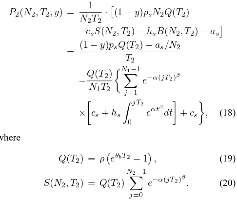
P2(N2, T2, y) = 1
N2T2 ·
[
(1−y)psN2Q(T2)
−csS(N2, T2)−hsB(N2, T2)−as
]
= (1−y)psQ(T2)−as/N2
T2
−Q(T2)
N1T2
{N∑1−1
j=1
e−α(jT2)β
×
[
cs+hs
∫ jT2
0
eαtβdt
]
+cs
}
, (18)
where
Q(T2) = ρ(eθbT2−1), (19)
S(N2, T2) = Q(T2)
N∑2−1
j=0
e−α(jT2)β. (20)
V. RETAILER’S OPTIMAL RESPONSE
This section discusses the retailer’s optimal response. The retailer prefers OptionV1 over OptionV2ifπ∗1> π2(T2, y), but when π∗1 < π2(T2, y), she/he prefers V2 to V1. The retailer is indifferent between the two options if π∗1 =
π2(T2, y), which is equivalent to
y =
(
ps+hθb
b
) [
Q(T2)−ρθbT2eθbT
∗ 1]+ab
psQ(T2)
. (21)
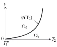
y
Ω1 Ω2
T2 (T 2)
ψ
[image:4.595.120.216.52.131.2]T1* 0
Fig. 2. Characterization of retailer’s optimal responses
VI. POULTRY FARMER’S OPTIMAL POLICY UNDER THE NON-COOPERATIVE GAME
The poultry farmer’s optimal values for T2 and y can be obtained by maximizing her/his total profit per unit of time considering the retailer’s optimal response which was discussed in Section V. Henceforth, let Ωi (i = 1,2) be
defined by
[image:4.595.318.548.198.376.2]Ω1 ={(T2, y)| y≤ψ(T2))}, Ω2 ={(T2, y)| y≥ψ(T2))}.
Figure 2 depicts the region ofΩi (i= 1,2) on the(T2, y) plane.
A. Under Option V1
If (T2, y)∈Ω1\Ω2 in Fig. 2, the retailer will naturally select Option V1. In this case, the poultry farmer can max-imize her/his total profit per unit of time independently of
T2 and y on the condition of (T2, y) ∈ Ω1\ Ω2. Hence, the poultry farmer’s locally maximum total profit per unit of time in Ω1\Ω2 becomes
P1∗ = max
N1∈N
P1(N1, T1∗), (22)
whereN signifies the set of positive integers.
B. Under Option V2
On the other hand, if (T2, y) ∈ Ω2\ Ω1, the retailer’s optimal response is to choose Option V2. Then the poultry farmer’s locally maximum total profit per unit of time in Ω2\Ω1 is given by
P2∗ = max
N2∈N
ˆ
P2(N2), (23)
where
ˆ
P2(N2) = max (T2,y)∈Ω2\Ω1
P2(N2, T2, y). (24)
More precisely, we should use ”sup” instead of ”max” in Eq. (24).
For a given N2, we show below the existence of the poultry farmer’s optimal quantity discount pricing policy (T2, y) = (T2∗, y∗) which attains Eq. (24). It can easily be proven that P2(N2, T2, y) in Eq. (18) is strictly decreasing iny, and consequently the poultry farmer can attainPˆ2(N2) in Eq. (24) by lettingy→ψ(T2) + 0. By letting y=ψ(T2) in Eq. (18), the total profit per unit of time on y =ψ(T2)
becomes
P2(N2, T2) = ρθb
(
ps+ hb θb
)
eθbT1∗− 1
N2T2
×
{
Q(T2)
[∑
N2−1
j=1 e−
α(jT)β
×(cs+hs
∫jT
0 e−
αtβdt)
+
(
N2hθb
b +cs
)]
+ (N2ab+as)
}
.(25)
By differentiatingP2(N2, T2)in Eq. (25) with respect to
T2, we have
∂ ∂T2
P2(N2, T2)
= − [
ρθbT2eθbT2−Q(T2)
]
×[(N2hθb
b +cs
)
+∑N2−1
j=1 e−
α(jT2)β
×(cs+hs
∫jT2
0 e−
αtβ
dt
)]
+Q(T2)T2
[
hs
N2(N2−1)
2
−r(T2)∑N2−1
j=1 j
βe−α(jT)β
×(cs+hs
∫jT2
0 e−
αtβdt)]
−(N2ab+as)
N2T22
.(26)
LetL(T2)express the terms enclosed in braces{ }in the right-hand-side of Eq. (26).
We here summarize the results of analysis in relation to the optimal quantity discount policy which attains Pˆ2(N2) in Eq. (24) whenN2 is fixed to a suitable value.
1) N2= 1:
In this subcase, there exists a unique finite To (> T1∗ ) which maximizes P2(N2, T2) in Eq. (25), and therefore(T2∗, y∗)is given by
(T2∗, y∗) → ( ˜T2, φ( ˜T2)), (27)
where
˜
T2 =
{
To, To≤Tmax/N2,
Tmax/N2, To> Tmax/N2.
(28)
The poultry farmer’s total profit then becomes
ˆ
P2(N2) = ρθb
[
(ps+hb/θb)eθbT ∗ 1
−(cs+hb/θb−α)eθbT ∗
2]. (29)
2) N2≥2:
Let us defineT2= ˜T2(> T1∗) as the unique solution (if it exists) to
L(T2) = (abN2+as). (30)
In this case, the optimal quantity discount pricing policy is given by Eq. (27).
C. Under OptionV1 andV2
TABLE I SENSITIVITY ANALYSIS
(a) Under OptionV1
cs Q∗1 p1 S1∗(N1∗) P1∗
35 71.64 100 71.64(1) 281.75 40 71.64 100 71.79(2) 265.82 45 71.64 100 71.79(2) 251.99 50 71.64 100 71.79(2) 238.17
(b) Under OptionV2
cs Q∗2 p∗2 S∗2(N2∗) P2∗
35 127.12 95.43 127.12(1) 310.24 40 123.95 95.81 123.95(1) 280.79 45 84.11 99.63 84.19(2) 254.73 50 84.11 99.63 84.19(2) 240.7
VII. POULTRY FARMER’S OPTIMAL POLICY UNDER THE COOPERATIVE GAME
This section discusses a cooperative game between the poultry farmer and the retailer. We focus on the case where the poultry farmer and the retailer maximize their joint profit. We here introduce some more additional notations N3, T3 and Q3, which correspond to N2, T2 and Q2 respectively, under OptionV2 in the previous section.
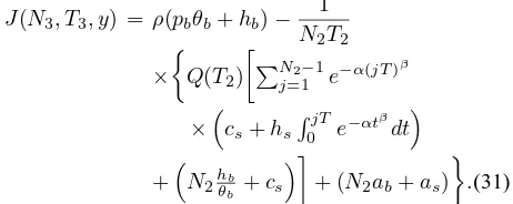
LetJ(N3, T3, y)express the joint profit function per unit of time for the poultry farmer and the retailer, i.e., let
J(N3, T3, y) =P2(N3, T3, y) +π2(T3, y), we have
J(N3, T3, y) = ρ(pbθb+hb)−
1
N2T2
×
{
Q(T2)
[∑
N2−1
j=1 e−
α(jT)β
×(cs+hs
∫jT
0 e−
αtβdt)
+
(
N2hθb
b +cs
)]
+ (N2ab+as)
}
.(31)
It can easily be proven from Eq. (31) that J(N3, T3, y) is independent of y and we have J(N3, T3, y) = P2(
N3, T3, ψ(T3)) +π∗1. This signifies that the optimal quan-tity discount policy (T3, y) = (T3∗, y∗) which maximizes
J(N3, T3, y) in Eq. (31) is given by (T2∗, y∗) as shown in Section VI. This is simply because, in this study, the inventory holding cost is assumed to be independent of the value of the item.
VIII. NUMERICAL EXAMPLES
Table I reveals the results of sensitively analysis in ref-erence to Q∗1, p1 (= ps), S1∗ (= S(N1∗, T1∗)), N1∗, P1∗,
Q∗2 (= Q(T2∗)), p∗2 (=(1 −y∗)ps), S∗2 (= S(N2∗, T2∗)),
N2∗,P2∗ for (ps, pb, as, ab, hs, hb, α, β, θb, µ, Tmax) = (100,
200,1000,1200,20,1,0.8,0.8,0.015,5,30) when cs = 35,
40,45,50.
In Table I(a), we can observe that Q∗1 takes a constant value (Q∗1 = 71.64). Under Option V1, the retailer does not adopt the quantity discount offered by the poultry farmer. The poultry farmer cannot therefore control the retailer’s ordering schedule, which signifies thatQ∗1 is independent of
cs. Table I(a) also shows thatS1∗increases whencsincreases
from 35 to 40 (more precisely, at the moment when cs
increases from 35.761 to 35.762). The weight of the fowl
increases as the breeding period increases. Under Option
V1, this period can be increased by means of increasing the number of the shipping cycle since the length of the retailer’s order cycle cannot be changed. Under this Option, when
cs takes a larger value, the poultry farmer should increase
her/his order quantity per lot to keep her/his fowls as long as possible.
Table I(b) indicates that, under OptionV2,Q∗2 is greater than Q∗1 (compare with Table I(a)). Under Option V2, the retailer accepts the quantity discount proposed by the poul-try farmer. The poulpoul-try farmer’s lot size can therefore be increased by stimulating the retailer to alter her/his order quantity per lot through the quantity discount strategy. We can also notice in Table I that we haveP1∗< P2∗. This indi-cates that using the quantity discount strategy can increase the poultry farmer’s total profit per unit of time.
IX. CONCLUSION
In this study, we have discussed a quantity discount prob-lem between a poultry farmer and a retailer for ameliorating items. These items include the fast growing animals such as broiler in poultry farm. The poultry farmer purchases chicks from an upper-leveled supplier and then feeds them until they grow up to be fowls. The retailer purchases (raw) chicken meat from the poultry farmer. The stock of the poultry farmer increases due to growth, in contrast, the inventory level of the retailer is depleted due to the combined effect of its demand and deterioration. The poultry farmer is interested in increasing her/his profit by controlling the retailer’s order quantity through the quantity discount strategy. The retailer attempts to maximize her/his profit considering the poultry farmer’s proposal. We have formulated the above problem as a Stackelberg game between the poultry farmer and the retailer to show the existence of the poultry farmer’s optimal quantity discount policy that maximizes her/his total profit per unit of time. In this study, we have also formulated the same problem as a cooperative game. The result of our analysis reveals that the poultry farmer is indifferent between the cooperative and non-cooperative options. It should be pointed out that our results are obtained under the situation where the inventory holding cost is independent of the value of the item. The relaxation of such a restriction is an interesting extension.
REFERENCES
[1] J. P. Monahan, “A quantity discount pricing model to increase vendor’s profit,” Management Sci., vol. 30, no. 6, pp. 720–726, 1984. [2] M. Data and K. N. Srikanth, “A generalized quantity discount pricing
model to increase vendor’s profit,” Management Sci., vol. 33, no. 10, pp. 1247–1252, 1987.
[3] M. J. Rosenblatt and H. L. Lee, “Improving pricing profitability with quantity discounts under fixed demand,” IIE Transactions, vol. 17, no. 4, pp. 338–395, 1985.
[4] H. L. Lee and M. J. Rosenblatt, “A generalized quantity discount pricing model to increase vendor’s profit,” Management Sci., vol. 32, no. 9, pp. 1177–1185, 1986.
[5] M. Parlar and Q. Wang, “A game theoretical analysis of the quantity discount problem with perfect and incomplete information about the buyer’s cost structure,” RAIRO/Operations Research, vol. 29, no. 4, pp. 415–439, 1995.
[6] S. P. Sarmah, D. Acharya, and S. K. Goyal, “Buyer vendor coordination models in supply chain management,” European Journal of Operational
Research, vol. 175, no. 1, pp. 1–15, 2006.
[image:5.595.62.293.393.485.2][8] B. Mondal and A. K. Bhunia, “An inventory system of ameliorating items for price dependent demand rate,” Computers & industrial
engi-neering, vol. 45, pp. 443–456, 2003.
[9] S. Y. Chou and W. T. Chouhuang, “An analytic solution approach for the economic order quantity model with weibull ameliorating items,”