Integrating stochasticity and network structure into an epidemic model

University of Warwick institutional repository:

http://go.warwick.ac.uk/wrap

This paper is made available online in accordance with

publisher policies. Please scroll down to view the document

itself. Please refer to the repository record for this item and our

policy information available from the repository home page for

further information.

To see the final version of this paper please visit the publisher’s website.

Access to the published version may require a subscription.

Author(s):

Dangerfield, C. E., Ross, J. V. and Keeling, M. J.

Article Title: Integrating stochasticity and network structure into an

epidemic model.

Year of publication: 2009

Link to published article : http://dx.doi.org/10.1098/rsif.2008.0410

Publisher statement: © Dangerfield, C. E., et al. This article has been

reproduced under a creative commons license attribution 3.0

doi: 10.1098/rsif.2008.0410

, 761-774 first published online 30 October 2008

6

2009

J. R. Soc. Interface

C. E. Dangerfield, J. V. Ross and M. J. Keeling

epidemic model

Integrating stochasticity and network structure into an

References

http://rsif.royalsocietypublishing.org/content/6/38/761.full.html#related-urls Article cited in:

http://rsif.royalsocietypublishing.org/content/6/38/761.full.html#ref-list-1 This article cites 38 articles, 13 of which can be accessed free

This article is free to access

Integrating stochasticity and network

structure into an epidemic model

C. E. Dangerfield

, J. V. Ross

and M. J. Keeling

*

1

Mathematics Institute, University of Warwick, Gibbet Hill Road, Coventry CV4 7AL, UK 2_{King’s College, University of Cambridge, Cambridge CB2 1ST, UK}

While the foundations of modern epidemiology are based upon deterministic models with homogeneous mixing, it is being increasingly realized that both spatial structure and stochasticity play major roles in shaping epidemic dynamics. The integration of these two confounding elements is generally ascertained through numerical simulation. Here, for the first time, we develop a more rigorous analytical understanding based on pairwise approximations to incorporate localized spatial structure and diffusion approximations to capture the impact of stochasticity. Our results allow us to quantify, analytically, the impact of network structure on the variability of an epidemic. Using the susceptible–infectious– susceptible framework for the infection dynamics, the pairwise stochastic model is compared with the stochastic homogeneous-mixing (mean-field) model—although to enable a fair comparison the homogeneous-mixing parameters are scaled to give agreement with the pairwise dynamics. At equilibrium, we show that the pairwise model always displays greater variation about the mean, although the differences are generally small unless the prevalence of infection is low. By contrast, during the early epidemic growth phase when the level of infection is increasing exponentially, the pairwise model generally shows less variation.

Keywords: noise; networks; pairwise moment closure; diffusion approximation

1. INTRODUCTION

From the early ordinary differential equation (ODE) compartmental models (Anderson & May 1983) to more recent spatially structured stochastic simulations (Riley 2007), models of infectious diseases have impacted on both our understanding of epidemic spread and public health planning. However, one of the key issues in using such models is a comprehensive under-standing of when complexity is important and when it is a superfluous detail. Here, we offer an analytical insight into the confounding roles of stochasticity and spatial structure in the dynamics of infection.

The chance nature of epidemiological processes can have a profound impact on disease dynamics, leading to a range of phenomena not predicted by deterministic models. Standard models based on ODEs are essentially clock work, predicting an identical outcome from the same initial conditions—in addition, such deterministic models generally predict constant endemic levels of infection in the long term (Anderson & May 1992;

Keeling & Rohani 2007). By contrast, by capturing the chance nature of transmission and recovery, stochastic models predict variability in the levels of infection. Such variability has two substantial consequences. Firstly, stochastic epidemics are prone to extinction either immediately following invasion (Bartlett 1956) or even once established (Bartlett 1957;Bolker & Grenfell 1995).

Secondly, the interaction of stochasticity with the natural oscillatory behaviour of epidemics can lead to large-scale oscillations—termed stochastic resonance (Dushoff et al. 2004; Alonso et al. 2006). The most common method of studying stochastic models is through simulations using techniques such as the Gillespie algorithm (Gillespie 1977); however, more recently analytical techniques such as moment closure approximations (Keeling 2000b;Na˚sell 2003), diffusion approximations (Clancy et al. 2001; Ross 2006) and exact Kolmogorov forward equations (Keeling & Ross 2008) have all been used to understand stochastic epidemic dynamics.

Spatial structure impacts on epidemic dynamics at a variety of scales. Humans generally live in relatively large communities (e.g. towns and cities) and this compartmentalization often induces spatial heteroge-neities, with strong transmission of infection within communities but weaker transmission between com-munities, capturing the general assumption that transmission strength decreases with separation (Xia

et al. 2004;Riley 2007). This large-scale heterogeneity has been captured in a wide number of contexts with both spatial (Gibson & Austin 1996; Keeling et al. 2001; Mangen et al. 2002; Ferguson et al. 2005) and metapopulation models (Bolker & Grenfell 1995;

Finkensta¨dt & Grenfell 1998; Smith et al. 2002;

Hanski & Gaggiotti 2004). However, at a more local scale the dynamics of infection are strongly influenced by the network of available contacts through which

*Author for correspondence ([email protected]).

doi:10.1098/rsif.2008.0410

J. R. Soc. Interface(2009)6, 761–774

infection can be transmitted. The use of network-based models to simulate the local spread of infection through social or sexual contacts has seen substantial advances over the past decade (Watts & Strogatz 1998;

Potterat et al. 1999; Klovdahl 2001; Halloran et al. 2002;Keeling & Eames 2005;Boccalettiet al. 2006). In general networks have three main influences over the epidemiological dynamics. Firstly, local connectedness and clustering leads to strong negative spatial corre-lations between infected and susceptible individuals rapidly leading to reduced transmission, reduced growth rate and therefore higher numbers of suscep-tibles at equilibrium (Keeling 2005). Secondly, hetero-geneities in the number of contacts automatically generate high- and low-risk individuals and hence heterogeneities in the distribution of infection (Eames & Keeling 2002; Keeling & Eames 2005). Finally, the long path length that may exist between individuals (Watts & Strogatz 1998) can lead to asynchronous behaviour across the network (Boots & Sasaki 1999). These three influences shape how individual-level epidemiological characteristics trans-late into population-level behaviour and hence are vitally important for predicting the impact of control measures, such as contact tracing, that are focused towards the individual (Eames 2007).

In this paper, we focus on bringing together two highly successful approximations—the diffusion approximation for stochastic populations and the pair-wise approximation for dynamics on a network—in order to understand the interaction between local spatial structure and stochasticity. In particular, we consider a susceptible–infectious–susceptible (SIS)-type model, which is a good description of many sexually transmitted infections (Anderson & May 1992;Andersson & Britton 2000;Keeling & Rohani 2007) and host–parasite diseases (Stone et al. 2008). Despite its applicability, the SIS model provides one of the simplest descriptions of disease transmission as individuals can be in only one of two states: susceptible or infectious.

We initially outline some relatively standard results: the dynamics of the deterministic (homogeneous-mixing or mean-field) SIS model (Anderson & May 1992); the Ornstein–Uhlenbeck (OU) diffusion approximation (Kurtz 1971) to the stochastic SIS model; and the deterministic pairwise equations for SIS-type infections spreading through a network (Eames & Keeling 2002). These results and the associated methodologies will then be combined to create a diffusion approximation to the stochastic pairwise SIS model and ultimately to calculate the associated variances and covariances. These results will be compared with those of two other stochastic models: the stochastic homogeneous-mixing SIS model and the full stochastic Monte Carlo (continuous-time Markov chain) network simulation.

2. BASIC METHODOLOGY

While the results and methodologies given below are described in far more detail in other publications, here we briefly summarize the techniques and salient results to more naturally lead the reader into the complexities that follow.

2.1. The deterministic SIS model

The simple SIS equation is one of the foundations of predictive models of sexually transmitted infections (Anderson & May 1992). Treating S and I as the

proportionof susceptible and infectious individuals in the population, and ignoring birth and death, the SIS equations are

dS

dt ZKbSICgI

dI

dtZbSIKgI

9 > > > > = > > > > ;

0dI

dt Zbð1KIÞIKgI; ð2:1Þ

where the single equation is derived from the fact that

SCIZ1. We note that if we wish to deal withnumbers

of susceptible and infectious individuals within the population then for consistency the transmission rateb

is divided by the total population sizeN;gis the rate at which individuals recover and move from the infectious to susceptible state. We refer to equation (2.1) as the deterministic mean-field model. The ability to switch between proportions and numbers will be vital when we consider integer-based stochastic models and their diffusion approximations. For the standard deter-ministic model it is easy to show that the non-trivial equilibrium point isI_Z1Kðg=bÞ, which is stable (and

the disease-free state is unstable) if the basic reproduc-tive ratioR0Zb=gis greater than 1 (Anderson & May 1992;Keeling & Rohani 2007).

2.2. Stochastic behaviour and the diffusion approximation

The above equations are however deterministic and deal only with the mean dynamics, and therefore do not capture the variability expected from any biological population. To account for this variability the dynamics are generally made stochastic, such that the population is integer-based and events occur at probabilistic rates. For the SIS equations, the stochastic counterpart is a Markovian process (future dynamics depend only on the current state) and hence a rich mathematical theory can be brought into play. Borrowing from the notation of pairwise models (Keeling et al. 1997), we define [S](ZNS) and [I](ZNI) to be thenumber of

suscep-tible and infectious individuals in the population. For a population of sizeN, we can now express the Markovian SIS system by defining the rate of transition between states (q(a,b) is the rate of transition from state a to stateb),

qð½I;½IClÞZ

Nb½I N 1K

½I N

0 @

1

A iflZC1;

Ng½I

N iflZK1:

8 > > > > > < > > > > > :

ð2:2Þ

population sizes or higher dimensional models—we therefore seek more robust analytical methods.

An extremely effective approach for studying stochastic dynamics, particularly when dealing with large population sizes, is to use diffusion approxi-mations. Such processes arise naturally in the frame-work of continuous-time Markov chains and provide a mathematically rigorous framework, which establishes conditions for convergence in the large population size limit (Kurtz 1970, 1971). Essentially, this framework allows us to replace the integer-based stochastic dynamics for the number of individuals by a stochastic (Gaussian) diffusion process in continuous space modelling the proportions of each state in the popu-lation. Moreover, exact analytic results can be for-mulated to describe the time evolution of variances and covariances within the system. Such models have been used to great effect in ecology (Ross 2006) and epidemiology (Clancyet al. 2001).

Given that for a fixed N (constant population size) the rates in equation (2.2) can be expressed solely in terms of proportions (i.e. ½I=N_ZI), then the (finite-state) Markovian SIS model is a density-dependent

process and satisfies the criteria for convergence to a Gaussian diffusion process (Kurtz1970,1971). For large population sizes this essentially has two main impli-cations: firstly, stochasticity can be captured by includ-ing appropriately scaled Gaussian noise to the dynamics and, secondly, the equilibrium dynamics converge to a Gaussian distribution whose variance can be calculated. More specifically, for the SIS model, the first implication means that the Markovian system can be accurately captured with a stochastic ODE model

dI

dtZbð1KIÞIKgIC

ffiffiffiffiffiffiffiffiffiffiffiffiffiffiffiffiffiffiffiffiffiffiffiffiffiffiffiffiffiffiffi

bð1KIÞICgI

N

r

xðtÞ; ð2:3Þ

wherexis the Gaussian white noise process with mean 0 and variance 1 (theorems 3.1 and 3.5, Kurtz 1971). Equation (2.3) effectively approximates the integer-based dynamics of equation (2.2) with a continuum-based model; in what follows we refer to equation (2.3) as the stochastic mean-field model (although readers may also prefer to consider this as the diffusion approximation to the stochastic mean-field SIS model) and equation (2.2) as the continuous-time Markov chain of the mean-field model.

The result of the second implication comes directly from the recognition that assuming the process is in equilibrium (that is assuming endemicity has been reached) we have an OU process, and thus the distribution around the equilibrium converges to a Gaussian with variance (Grimmett & Stirzaker 2001)

VarðIÞZK

bIð1KIÞCgI

2ðbð1K2IÞKgÞN Z

g

bNZ

1

R0N

Z

1KI

N : ð2:4Þ

When considering the number of infectious individuals, [I], the variance scales to Varð½IÞZNðg=bÞ; the fact

that the number of infected individuals and the associated variance both scale linearly with population size (for large N) agrees with a range of simulation

results and biological findings (Taylor 1961; Keeling 2000a). The above calculations follow the more general methodology given in appendix B. We note that, for such processes and in the large population size limit, the mean of the stochastic process and the deterministic equilibrium are equal.

2.3. Pairwise approximations

Pairwise approximation models offer a relatively low-dimensional and parsimonious means of extending standard ODE disease models to incorporate network structure (Keeling 1999; Keeling & Eames 2005). For sexually transmitted infections where the transmission network of sexual contacts generally has limited clustering, the pairwise approximation has been found to produce results in good agreement with network-based simulations, although due to its deterministic nature the pairwise equations are unable to explain the observed variability (Eames & Keeling 2002). Although more complex versions of the pairwise equations have been developed to capture the observed heterogeneity in the number of sexual partners (Eames & Keeling 2002), for simplicity in this paper we deal with the pairwise approximation to a regular network (Caley tree) where every individual has exactly

n contacts (Keeling 1999). We stress that this is an approximation to the observed highly heterogeneous nature of sexual contact networks, but it allows us to develop a relatively low-dimensional description of the infectious dynamics as individuals are homogeneous.

Using the notation developed by Rand and co-workers (Keeling et al. 1997) and described in detail elsewhere (Keeling 1999), we find that, for an SIS-type infection, the number of infectious individuals is determined by

d½I

dt Zt½SIKg½I; ð2:5Þ

where [I] is the number of infectious individuals in the population and [SI] is the number of susceptible– infectious pairs—noting that pairs are counted in both directions and that [SI]_Z[IS]. In this equation, the transmission occurs at a rate t across any contact between an infectious individual and a susceptible individual, hence including the network structure; more-over, equation (2.5) is an exact description of the deterministic dynamics if we know the number ofS–I

pairs. One approach is to approximate the number of

S–Ipairs from the number of susceptible and infectious individuals in the population assuming that the constitu-ents of the pair are uncorrelated ([SI]z[S]$[I]/N); this

is the random-mixing assumption and leads to the basic SIS model (equation (2.1)). The alternative approach is to formulate equations for the pairs [SI] and [II], which leads to the following coupled ODEs:

d½SI

dt Zt½SSICg½IIKt½SIKt½ISIKg½SI;

d½II

dt Z2t½ISIC2t½SIK2g½II:

9 > > > > = > > > > ;

These equations are based on the rates at which particular pair types are created or destroyed; for example, the first term in the first equation relates to the creation of an

S–Ipair from anS–Spair which is part of anS–S–Itriple. (A more complete description of this type of formulation is given in Keeling (1999).) We note that again these pairwise equations offer an exact description of the SIS epidemic process on a network, although the formulae require knowledge of the number of triples (e.g. [SSI]) in the population. Using the now standard approach (Keeling 1999), we approximate the number of triples in terms of the number of pairs, assuming the network is a regular random graph—everyone has n contacts and these are chosen at random from the population,

½ABCzðnK1Þ

n

½AB½BC

½B : ð2:7Þ

Essentially, this approximation considers a triple to be composed of two pairs that share the central individual but are otherwise independent.

The standard deterministic pairwise model (equation (2.6)) deals with numbers of pairs within the population. To make the scaling within our formalism more precise, we define two new variables,

uandv, which lie between 0 and 1, and which measure the proportion of pairs of typeS–IandI–I,respectively (u_Z[SI]/(nN),v_Z[II]/(nN)0uCvZI). Hence, using

the triple approximation (equation (2.7)), the pairwise SIS model can be written in full as,

du

dt ZtðnK1Þ

uð1K2uKvÞ

1KuKv CgvKtuKtðnK1Þ

u2

1KuKv Kgu;

dv

dt Z2tðnK1Þ u2

1KuKv

C2tuK2gv:

9 > > > > > > = > > > > > > ;

ð2:8Þ

The aim of this paper is now to capture the variability about the solution of equations (2.6) or (2.8) using coupled stochastic ODEs (i.e. a diffusion approxi-mation), and in particular to extract the variance– covariance matrix for this system. Both of these operations can be achieved using standard approaches given that the stochastic formulation of (2.6), combined with (2.7), defines a density-dependent process and satisfies the criteria for convergence to a Gaussian distribution (Kurtz1970,1971).

From equation (2.8) it is relatively easy to determine the equilibrium (endemic level of infection)

uZ

rðnK1ÞK1

rðr nðnK1ÞK1Þ

vZ

rðnK1ÞðrðnK1ÞK1Þ

rðr nðnK1ÞK1Þ

;

whererZt/gmust be greater than 1/(nK1) andnR2,

otherwise the disease always dies out. We therefore see thatr(nK1) has a close analogy toR0in standard

(non-network) disease models.

In the calculations that follow, in order to achieve a fair comparison between the mean-field SIS model (equation (2.1)) and our pairwise model (equation (2.6) or (2.8)), we insist that both models have the same proportion of infectious individuals at equilibrium

Ipairwise ZuCvZ

nðrðnK1ÞK1Þ

ðr nðnK1ÞK1ÞZ

I_ZbKg b

0rZ

R₀ðnK1ÞC1

nðnK1Þ

;

which, as expected, provides agreement at the threshold for successful invasion (R0Z10r(nK1)Z1).

3. STOCHASTIC ODEs FOR THE SIS PAIRWISE MODEL

Conversion of the integer-based stochastic pairwise model to its stochastic diffusion approximation should in principle be relatively straightforward, adding a scaled Gaussian noise term for each event that can occur. However, great care is needed in determining precisely the nature of each possible event. For SIS-type disease dynamics only two processes occur— infection and recovery. In the mean-field stochastic model each of these processes is associated with a single event, changing the number of infectious and suscep-tible individuals by one. However, for a pairwise-based approach, it becomes necessary to consider the entire neighbourhood surrounding the affected individual, this is because infection and recovery can cause a variety of changes to the number of pairs dependent on the constituents of the neighbourhood. For example, consider an infectious individual whose neighbourhood consists ofmother infected individuals and hencenKm

susceptibles; if this central infectious individual recovers then m II pairs and (nKm) SI pairs are

destroyed, but m SI pairs and (nKm) SS pairs

are created. From this argument it is clear that we must consider as separate events each process and each neighbourhood configuration. This is a considerable conceptual change. Previously, the pairwise model (as the name suggests) focused on the dynamics of pairs of connected individuals that often necessitated calcu-lation of connected triples but higher order neighbour-hood configurations could be ignored; however, the stochastic version of this model while still focusing on the dynamics of pairs requires the consideration of the entire neighbourhood of an individual. This change of perspective may make it easier to include the effects of heterogeneities and local clustering within the network structure. Under this reformulation, the standard pairwise equations (2.6) become:

d½SI

dt Z½S Xn

mZ0

n

m !

½SI

n½S

m

1K

½SI

n½S

nKm

( )

!ftmgfðnKmÞKmg

C½I

Xn

mZ0

n

m !

½II

n½I

m

1K

½II

n½I

nKm

( )

!fggfmKðnKmÞg;

d½II

dt Z½S Xn

mZ0

n

m !

½SI

n½S

m

1K

½SI

n½S

nKm

( )

!ftmgf2mg

C½I

Xn

mZ0

n

m !

½II

n½I

m

1K

½II

n½I

nKm

( )

!fggfK2mg:

9 > > > > > > > > > > > > > > > > > > > > > > > > > > > = > > > > > > > > > > > > > > > > > > > > > > > > > > > ;

The three elements in braces for each term refer to: the probability of having m infectious individuals around the central node (assuming pairwise correlation but uncorrelated triples); the rate at which the event occurs given the neighbourhood; and the change to the number of pairs given the neighbourhood. This new formulation (equation (3.1)) essentially operates at the scale of neighbourhoods surrounding central individuals, but uses the pairwise correlation information to construct these in a weighted manner, although correlations between neighbours and within triples are ignored. We note that, as expected, when the sums in equation (3.1) are evaluated we regain equation (2.6).

The formulation of a stochastic ODE approximation accounting for the variation about equations (3.1) proceeds as before, with each event (corresponding to each neighbourhood configuration and each process) associated with an additional noise term. The full set of stochastic ODEs is shown in appendix A, from which we observe that we can either construct the stochastic ODEs by including one scaled noise term for each event (Keeling & Rohani 2007) or we can use the methods developed by Kurtz (1970, 1971) to construct a 2!2

covariance noise matrix. These two approaches agree due to the independence of the noise terms that arise from considering events rather than processes. An example of aggregated results from numerically inte-grating equations (A 1) or (A 2) is given infigure 1; note that as expected the mean of the two stochastic ODEs (equations (2.3) and (A 1) or (A 2)) agree and is equal to the deterministic mean. Fromfigure 1a, we observe comparatively close agreement between the stochastic pairwise and stochastic mean-field results in terms of the variance in the total number of infectious individ-uals, [I]—noting that the transmission parameter of the stochastic model has been rescaled to achieve agreement in the deterministic equilibrium. The pair-wise model has a slightly higher variance and this is found to be a consistent feature of all parameter regimes tested. Figure 1b,c provides more insight into the constituent pairwise components of this variation. Firstly, we note the negative correlation between the proportion of S–I pairs (x-axis) and the proportion ofI–I pairs or the proportion of infectious individuals (y-axis). In addition, for these parameters, the variation associated with S–I pairs is far less than the variation in I–I pairs, and so it is this latter variation that drives the overall variance in the level of infection.

While equations (A 1) and (A 2) in appendix A provide a means of numerically integrating the sto-chastic dynamics of the pairwise equations, they do not provide an easy analytical comparison with the results derived for the stochastic SIS model (equation (2.4)). We therefore use equation (2.8) together with the standard results for OU processes (Grimmett & Stirzaker 2001) to derive the distributions around the mean equilibrium value for large population sizes. The full covariance matrix for the variables u and v

is cumbersome and consequently not overly inform-ative (see appendix B). We therefore focus primarily on the variance in the proportion of the population that are infectious, and undertake numerical comparisons

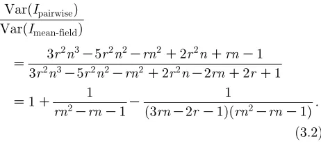
between the stochastic mean-field SIS model and the stochastic pairwise equations to inform about the interactions between noise and network processes. The variance from the pairwise model is given by:

VarðIpairwiseÞ

Zð

nK1Þð3r2n3K5r2n2Krn2C2r2nCrnK1Þ

Nð3rnK2rK1Þðrn2KrnK1Þ2

;

whereas, for the mean-field model (assuming the same equilibrium value), we have

VarðImean-fieldÞZ

ðnK1Þ

Nðrn2

KrnK1Þ

:

Examining the ratio of the two variances we find that:

VarðIpairwiseÞ

VarðImean-fieldÞ

Z 3r

2_n3

K5r2n2Krn2C2r2nCrnK1

3r2n3K5r2n2Krn2C2r2nK2rnC2rC1

Z1C

1

rn2

KrnK1 K

1

ð3rnK2rK1Þðrn2KrnK1Þ

:

ð3:2Þ

Hence, the stochastic pairwise model always has a greater variance than the stochastic mean-field model, but the ratio drops to 1 as eitherr,n or R0becomes

large. In part this is to be expected as the mean-field model can be considered as the limiting case of the pairwise model asnbecomes large, and hence we would expect agreement. Whenris relatively large, then both models predict that most of the population is infected leading to little spatial structure within the network (as captured by the pairwise equations) and so the stochastic mean-field model is an accurate approxi-mation to the full dynamics.

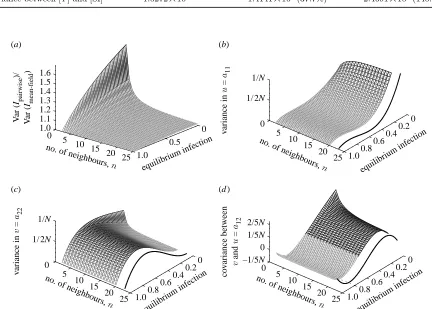
Figure 2 shows the bivariate normal distribution for various combinations of the key parameters, which should be compared with the numerical results from the stochastic version of the pairwise and mean-field models shown in figure 1. These results confirm our earlier findings and validate the analytical calcu-lations given in the appendices. The close agreement between the stochastic mean-field (thick black line) and stochastic pairwise (shaded area) models, in terms of variation in the number of infectious individuals, is particularly striking. For the par-ameters used in figures 1 and 2, table 1 details the numerical values of various quantities of interest for both the stochastic pairwise model and the mean-field equivalent. For completeness results from a full Monte Carlo network simulation are also given in

equilibrium level of infection. In particular, the deviation between the stochastic mean-field and the full Monte Carlo network simulation is generally far greater than the deviation between the pairwise model and the network simulation; most strikingly

the variance in S–I pairs is poorly captured by the stochastic mean-field approximation.

Figure 3extends the above analysis across a range of parameter values; in particular, as the number of neighboursnand the equilibrium (endemic) level of infectionIvaries. From all these figures it is clear that the maximum deviation from the stochastic mean-field results (shown as a thick black line) occurs when the number of contacts, n, is small and when the equilibrium level of infection is low. It is also apparent that the convergence to mean-field happens rapidly with increasingn. As expected, the ratio of the pairwise variance in the level of infection to the mean-field

5.450 5.50 5.55 5.60 5.65 0.2

0.4 0.6 0.8 1.0 1.2 1.4 1.6 1.8 2.0 (a)

(b)

(c)

no. of infected, [×10 4 I ]

frequenc

y

[×10

–3]

proportion

I–

I pairs,

v

= [II]/

n

N

0.324 0.326 0.328 0.330 0.332 0.334 0.336 0.338 0.340 0.342 0.344

frequenc

y (% of max)

1 10 20 50 90

frequenc

y (% of max)

1 10 20 50 90

proportion S–I pairs, u = [SI]/nN

proportion infected,

I

0.220 0.225 proportion S–I pairs, u = [SI]/nN

0.220 0.225

0.545 0.550 0.555 0.560

Figure 2. Distributions from the bivariate normal distri-butions predicted from the dynamics of the stochastic SIS pairwise (black bars) and mean-field (white bars) models (equation (2.4) and appendix B). Graphs and parameters are exactly as in figure 1 for ease of comparison. (b) and (c) show the 1, 10, 20, 50 and 90% contours.

5.45 5.50 5.55 5.60 5.65 0

0.01 0.02 0.03 0.04 0.05 0.06 0.07 0.08 0.09 0.10 (a)

(b)

(c)

no. of infected, [×104 I ]

frequenc

y

0.220 0.225 0.324

0.326 0.328 0.330 0.332 0.334 0.336 0.338 0.340 0.342 0.344

0.220 0.225

frequenc

y (% of max)

0 10 20 30 40 50 60 70 80 90 100

frequenc

y (% of max)

0 10 20 30 40 50 60 70 80 90 100

0.545 0.550 0.555 0.560

proportion of infected,

I

Figure 1. Distributions from the stochastic ODEs (equations (2.3), (A 1) and (A 2)). (a) compares the distribution of the number of infectious individuals from stochastic pairwise (black bars) and mean-field (white bars) versions of the SIS model; the pairwise model can be seen to give rise to a slightly larger variation. (b) and (c) are from the stochastic pairwise model only, and consider the covariance between the proportion ofS–Ipairs and either the proportion ofI–I

pairs or the proportion of the population that is infectious. Here, proportions are used such that axes can be plotted on equal scales, and we plot the frequency as a percentage of the maximum for ease of comprehension. (tZ0.05,gZ0.01, nZ5, NZ100 0000rZ0.5, R0Z2.25, bZ0.225, IZ5/9.

variance shows that the pairwise model always experi-ences greater variability (figure 3a)—with the ratio tending to 5/3 whennZ2 and asI/0. For each of the

figure 3b–d, the stochastic mean-field results (shown as thick black lines) that are equivalent to the largenlimit of the stochastic pairwise model can be calculated in terms of the equilibrium level of infection and the

stochastic mean-field variance:

VarðuÞZa11Zð1K2IÞ2VarðImean-fieldÞ;

VarðvÞZa22Z4I 2

VarðImean-fieldÞ;

Covarðu;vÞZa12Z2I

ð1K2IÞVarðImean-fieldÞ;

Table 1. Comparison of key distributional values for a full Monte Carlo (continuous-time Markov chain) network simulation, the stochastic pairwise and the stochastic mean-field models. (The network simulation uses full asynchronous updating of the disease status of each node (Gillespie 1977;Keeling & Eames 2005;Keeling & Rohani 2007), a regular network where each node has five contacts. The network simulation and pairwise model share the same individual-level parameters (tZ0.05,gZ0.1,nZ5, NZ100 000), while the mean-field model is again parametrized to have the same equilibrium level of infection as the pairwise model. The pairwise results come from the covariance matrix calculated in appendix B. The stochastic mean-field model is parametrized to have the same equilibrium level of infection, while the pairwise values (for the mean-field model) are calculated making the mean-field assumption of ignoring spatial correlation within the pair. The values in brackets show the percentage deviation of the stochastic pairwise and mean-field results away from the simulated values; clearly the pairwise model consistently performs better.)

quantity

Monte Carlo network simulation

stochastic pairwise (% deviation)

stochastic mean-field (% deviation)

mean number infected, [I] 5.4993!104 5.5556!104(1.0%) 5.5556!104(1.0%)

mean numberI–Ipairs, [SI] 1.0997!105 1.1111!105(1.0%) 1.2346!105(12.3%)

mean numberI–Ipairs, [II] 1.6500!105 1.6667!105(1.0%) 1.5432!105(6.5%)

variance in [I] 5.0057!104 4.8485!104(3.1%) 4.4444!104(11.2%)

variance in [SI] 7.1892!104 6.6667!104(7.3%) 1.3727!104(80.9%)

variance in [II] 1.4262!106 1.4202!106(0.4%) 1.3718!106(3.8%)

covariance between [I] and [SI] K1.0272!104 K1.4141!104(37.7%) K2.4691!104(140.4%)

0 0.5 1.0 0 ₅

10 15 ₂₀

25 1.0

1.1 1.2 1.3 1.4 1.5 1.6

equilibrium infection

equilibrium infection equilibrium infection

equilibrium infection no. of neighbours,

n

no. of neighbours,

n

no. of neighbours,

n no. of neighbours,

n

V

ar (

Ipairwise

)/

V

ar (

Imean-f

ield

)

0 0.2 0.4 0.6 0.8 1.0 0

5 10

15 20

25 1/ 2N

1/N

v

ariance in

u

=

a11

0 0.2 0.4 0.6 0.8 1.0 0

5 10

15 20

25 1/ 2N

1/N

v

ariance in

v

=

a22

0 0.2 0.4 0.6 0.8 1.0 0

5 10

15 20

25 –1/5N

0 1/5N 2/5N

co

v

ariance between _v and

u

=

a12

(a) (b)

(c) (d )

Figure 3. Comparison of stochastic pairwise and mean-field results using the predicted bivariate normal distributions. All graphs are plotted for a range of equilibrium infection levels (0!I!1) and for the various numbers of contacts (2%n%20); we equate equilibrium levels rather than transmission rates as this gives a more natural interpolation between pairwise and mean-field results. In (b–d), the thick black line gives the largenlimit of the pairwise model calculated from the predicted mean-field variance. (a) shows the relative variance in the level of infection for the stochastic pairwise model compared with the stochastic mean-field, Var(Ipairwise)/Var(Imean-field) (equation (3.1)); (b–d) show the variance in u, the variance invand the covariance

where the variance in the level of infection Var(Imean-field)

Z(1KI)/N. Examining figure 3b,c, we observe that,

whenever the equilibrium level of infection is relatively high (greater than 0.2) or when n is very small, the variance inv(associated withI–Ipairs) dominates the variance in u (associated with S–I pairs), and hence contributes the most to the variance in the level of infection; this is the case for the parameters in figures 1and2. Finally, infigure 3d, we consider the covariance between u and v and note that, although the precise value of this covariance changes withn, the point where the covariance is 0 always occurs atIZ1/2.

4. VARIANCE DURING EARLY GROWTH

The above comparisons have all used methodologies developed for the long-term stochastic dynamics around the equilibrium. However, comparable, but more complex, formulae exist (appendix C) that deal with variation about temporally varying population dynamics. We use this formalism to examine the dynamics following invasion in the particular case where both deterministic and pairwise SIS models predict exponential growth of infection at rate k

(e.g.I(t)ZI(0)exp(kt)). For the model we find thatkZ

bKgand hencekis positive wheneverR0is greater than

1. For the pairwise model the calculation of early growth rates is more complex; either we can use an eigenvalue approach on the SIS system of equations (2.6) or we can note that [SI] and [II] (or equivalentlyuandv) must also grow at ratek and calculate their ratio. In either case, exponential growth occurs only once initial transient dynamics have died away and a consistent spatial structure has developed (setting the ratio of [SI] to [II];

Keeling 1999). We equilibrate the exponential growth rates, rather than simplyR0, for two reasons: firstly, this

fitting ensures that (after transients) the two determi-nistic models have identical early behaviour and, secondly, because it is the early growth rate of an epidemic that is measured in practice.

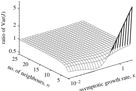
The results in appendix C therefore provide an analytical understanding of the variation about the expected exponential growth rate of infection once initial transient dynamics have decayed. We first note that both stochastic mean-field and stochastic pairwise models predict that the variance grows such as exp(2kt); or equivalently that the standard deviation (square root of the variance) grows at the same rate as infection. A comparison between the relative variances predicted by stochastic mean-field and stochastic pairwise models is shown in figure 4; this should be compared with figure 3a, which shows similar relative variances at equilibrium. Three main conclusions can be drawn. Firstly, for the majority of parameter space the variance predicted by the stochastic pairwise model is less than that predicted by the mean-field equivalent; the only exception occurs whennZ2 and the growthk

is large. The anomalous behaviour occurs because when

n_Z2 the network is reduced to a simple line; this places strong constraints on the early growth of infection such that kwpffiffiffit, whereas when nO2 we find that kwt

(appendix C). Secondly, for each value of n there is a growth rate kmin (close to the recovery rate, g) that

minimizes the relative variance in the pairwise model. Finally, because we have forced both models to agree on the population-level dynamics (by fixing the early growth rate) we again find that the predictions of stochastic mean-field and pairwise models are in far closer agreement than if we had simply matched the individual-level behaviour.

5. DISCUSSION

Three main conclusions can be drawn from this work. The first is that, with careful separation of all possible events (as opposed to processes), it is relatively straightforward to consider how stochasticity influ-ences the dynamics of pairwise models and hence how stochasticity and local spatial structure interact. The separation of events effectively leads us to work with neighbourhoods of individuals (rather than connected pairs) and use the pairwise correlations to define the distribution of neighbourhood types—assuming neighbours are independent leading to a multinomial distribution of neighbourhoods. This is a considerable conceptual change from the standard pairwise models that deal solely with contacts; the ability to deal with entire neighbourhoods opens up the possibility to consider far more complex network structures centred on individuals.

The second, more striking, conclusion is that for the vast majority of parameter space the stochastic pairwise model and (a suitably parametrized) stochas-tic mean-field model have very similar variation in the total level of infection close to the endemic equilibrium. We now speculate as to why this occurs. Consider the deterministic mean-field and pairwise equations, for-mulated for the number of infectious individuals,

10–2

1

5 10 15 20 25 0.5

1 2 5

asymptotic growth rate,

ratio of Var(

I)

Figure 4. Comparison of stochastic pairwise and mean-field results using the predicted bivariate normal distributions for the stochastic dynamics during the early exponential growth phase following invasion into a totally susceptible population. In particular, we compare the variance in the level of infection (Var(Ipairwise(t))/Var(Imean-field(t)); appendix C), when both

deterministic and pairwise models are parametrized to have a growth ratek. Lines are pale grey when the ratio is less than 1 and black when the ratio is more than 1. (Here, we setgZ0.1,

d½I

dt Zb½S½I=NKg½I

d½I

dt Zt½SIKg½I:

When these two models are parametrized to have equal levels of infection at equilibrium, it is clear that

b[S][I]/NZt[SI]. Given that the noise associated

with the level of infection (e.g. equation (2.3)) is defined in terms of the rates of change, the instan-taneous noise experienced by the stochastic mean-field and pairwise model at equilibrium must be identical. Therefore, the only source of variation between the two models is the deviation of t[SI] away from

b[S][I]/N. Examining the correlation between [SI] and [I], which is captured bys2₁₁Cs222 (appendix B),

shows only a relatively slight deviation between the stochastic pairwise model and the mean-field limit. Additional deviation may be caused by the noise associated with the [SI] term, whereas in the mean-field limit this term is proportional to the variation in the level of infection; however, in the large population size limit that we are considering here such effects are small. We therefore conclude that, except when both the number of contacts and the equilibrium level of infection are small, the act of forcing the two deterministic models to have equal equilibria leads to equal rates of infection and recovery at the equilibrium, which in turn leads to comparable levels of noise being experienced by the stochastic version of these models. Of course, the pairwise model also experiences noise in the correlation between connected individuals, but the impact of this on the dynamics is minimal when the population size is large.

Given this similarity in the level of variation predicted for stochastic pairwise and stochastic mean-field models, the usefulness of these results (and network/pairwise models in general) may be ques-tioned; however, we believe that these models are both useful and informative. A wide body of literature has demonstrated that network models can generate very different dynamics compared with the mean-field equivalent (Keeling & Eames 2005; Boccaletti et al. 2006); however, stochastic differences have rarely been elucidated. The similarity in stochastic variation observed here is both non-intuitive and critically dependent on our careful matching of the mean dynamics. We therefore feel that the development of the stochastic pairwise methodology is both informa-tive and likely to have significant applied impact when used to consider more complex network constructions that include heterogeneity and clustering.

The final conclusion concerns the early dynamics following invasion. Here, except for the anomalous case whenn_Z2, the stochastic pairwise model is predicted to have a lower variance than its mean-field counter-part; with the relative difference being greatest when the number of contactsnis small and the growth ratek

is comparable with the recovery rate g. As with the variance around the equilibrium, the relative differences between mean-field and pairwise predictions are not huge and generally are within a factor of two—the same reasoning as above still holds given that we are now forcing both models to have the same exponential growth rate. We speculate that spatial

structure has a stabilizing effect (lower variance) during the exponential growth phase because there is negative feedback via the spatial correlation captured by S–I

pairs; an infectious individual who by chance infects more of its contacts than expected depletes its local environment of susceptibles and therefore its sub-sequent chance of generating further cases is reduced. Simply put, for the regular network considered here, each infectious individual is limited to cause at mostn

secondary cases which in turn limit the noise associ-ated with each generation compared with the mean-field approximation.

In summary, if we assume that network and mean-field models are parametrized to match the same epidemic growth rate data, then the lower variation predicted in the stochastic version of the pairwise model (compared with the stochastic mean-field model) is likely to lead to a lower level of stochastic extinction in the pairwise model. We therefore postu-late that stochastic network-based models should be easier to invade (be less prone to early stochastic extinction) than their stochastic mean-field counter-parts, although their latter dynamics are subject to larger fluctuations.

In this paper, we have concentrated on developing a standard formulation within which noise can be incorporated into the pairwise modelling approach in a manner that scales appropriately with the rates at which events occur. We have taken the simplest of epidemiological models—the SIS model and the simplest network structure—a random network in which each individual has exactly n contacts. Many subsequent improvements to this general approach remain to be made. The methodology could equally be applied to the alternative pairwise formulation of Boots & Sasaki (1999, 2002) to provide insights into noise on lattice-based models. While the SIS para-digm is a good approximation for sexually trans-mitted infections and many host–parasite diseases, other epidemiological models could be considered, such as SIR or SEIR type dynamics; however, given the similarity in the infection equation for all these models we again expect stochastic pairwise and suitably parametrized stochastic mean-field models to experience relatively similar levels of variability. Of more importance is heterogeneity and clustering within the network structure—we speculate that having some highly connected (high-risk) individuals within the population or having the population composed of tightly interconnected groups is likely to impact substantially on the level of noise experi-enced. Bringing together the existing formalism to deal with heterogeneous or clustered pairwise models (Keeling 1999; Eames & Keeling 2002) with the method of including noise outlined in this paper is clearly possible but remains a challenge for the future.

APPENDIX A. STOCHASTIC ODE MODEL FOR THE PAIRWISE EQUATIONS

d½SI

dt Z½S

Xn

mZ0 n

m

!

½SI n½S

0 @ 1 A m 1K ½SI n½S

0 @ 1 A nKm 8 < : 9 =

;ftmgfðnKmÞKmg

C

Xn

m_Z0

ðnK2mÞ

ffiffiffiffiffiffiffiffiffiffiffiffiffiffiffiffiffiffiffiffiffiffiffiffiffiffiffiffiffiffiffiffiffiffiffiffiffiffiffiffiffiffiffiffiffiffiffiffiffiffiffiffiffiffiffiffiffiffiffiffiffiffiffiffiffiffiffiffiffiffiffiffiffiffiffiffiffiffi

½S n m

!

½SI n½S

0 @ 1 A m 1K ½SI n½S

0 @ 1 A nKm tm v u u u

t xmðtÞ

C½I

Xn

mZ0 n

m

!

½II n½I

0 @ 1 A m 1K ½II n½I

0 @ 1 A nKm 8 < : 9 =

;fggfmKðnKmÞg

C

Xn

mZ0

ð2mKnÞ

ffiffiffiffiffiffiffiffiffiffiffiffiffiffiffiffiffiffiffiffiffiffiffiffiffiffiffiffiffiffiffiffiffiffiffiffiffiffiffiffiffiffiffiffiffiffiffiffiffiffiffiffiffiffiffiffiffiffiffiffiffiffiffiffiffiffiffiffiffiffiffiffiffi

½I n m

!

½II n½I

0 @ 1 A m 1K ½II n½I

0 @ 1 A nKm g v u u u

t zmðtÞ;

d½II

dt Z½S

X

mZ0

n n

m

!

½SI n½S

0 @ 1 A m 1K ½SI n½S

0 @ 1 A nKm 8 < : 9 =

;ftmgf2mg

C

Xn

mZ0

2m

ffiffiffiffiffiffiffiffiffiffiffiffiffiffiffiffiffiffiffiffiffiffiffiffiffiffiffiffiffiffiffiffiffiffiffiffiffiffiffiffiffiffiffiffiffiffiffiffiffiffiffiffiffiffiffiffiffiffiffiffiffiffiffiffiffiffiffiffiffiffiffiffiffiffiffiffiffiffi

½S n m

!

½SI n½S

0 @ 1 A m 1K ½SI n½S

0 @ 1 A nKm tm v u u u

t xmðtÞ

C½I

Xn

mZ0 n

m

!

½II n½I

0 @ 1 A m 1K ½II n½I

0 @ 1 A nKm 8 < : 9 =

;fggfK2mg

C

Xn

mZ0

ðK2mÞ

ffiffiffiffiffiffiffiffiffiffiffiffiffiffiffiffiffiffiffiffiffiffiffiffiffiffiffiffiffiffiffiffiffiffiffiffiffiffiffiffiffiffiffiffiffiffiffiffiffiffiffiffiffiffiffiffiffiffiffiffiffiffiffiffiffiffiffiffiffiffiffiffiffi

½I n m

!

½II n½I

0 @ 1 A m 1K ½II n½I

0 @ 1 A nKm g v u u u

t zmðtÞ;

9 > > > > > > > > > > > > > > > > > > > > > > > > > > > > > > > > > > > > > > > > > > > > > > > > > > > > > = > > > > > > > > > > > > > > > > > > > > > > > > > > > > > > > > > > > > > > > > > > > > > > > > > > > > > ;

ðA 1Þ

where xm and zm are independent Gaussian white noise processes (mean 0 and variance 1) associated with

transmission and recovery, respectively.

This can also be expressed with the formulation by Kurtz (1970), which generates a somewhat simpler set of equations:

d½SI

dt Z½S

Xn

mZ0 n

m

!

½SI n½S

0 @ 1 A m 1K ½SI n½S

0 @ 1 A nKm 8 < : 9 =

;ftmgfðnKmÞKmg

C½I

Xn

m_Z0 n

m

!

½II n½I

0 @ 1 A m 1K ½II n½I

0 @ 1 A nKm 8 < : 9 =

;fggfmKðnKmÞgCA11xðtÞCA12zðtÞ;

d½II

dt Z½S

X

mZ0 n

m

!

½SI n½S

0 @ 1 A m 1K ½SI n½S

0 @ 1 A nKm 8 < : 9 =

;ftmgf2mg

C½I

Xn

mZ0 n

m

!

½II n½I

0 @ 1 A m 1K ½II n½I

0 @ 1 A nKm 8 < : 9 =

;fggfK2mgCA21xðtÞCA22zðtÞ;

9 > > > > > > > > > > > > > > > > > > > > > = > > > > > > > > > > > > > > > > > > > > > ;

ðA 2Þ

H_11ZX

n

mZ0

½S n m

!

½SI n½S

0 @ 1 A m 1K ½SI n½S

0 @ 1 A nKm 8 < : 9 =

;ftmgðnK2mÞ

2

0 @

C½I

n

m

!

½II n½I

0 @ 1 A m 1K ½II n½I

0 @ 1 A nKm 8 < : 9 =

;fggð2mKnÞ

2

1 A;

H12ZH21Z

Xn

mZ0

½S n m

!

½SI n½S

0 @ 1 A m 1K ½SI n½S

0 @ 1 A nKm 8 < : 9 =

;ftmgðnK2mÞð2mÞ 0

@

C½I

n

m

!

½II n½I

0 @ 1 A m 1K ½II n½I

0 @ 1 A nKm 8 < : 9 =

;fggð2mKnÞðK2mÞ 1 A;

H22Z

Xn

mZ0

½S n m

!

½SI n½S

0 @ 1 A m 1K ½SI n½S

0 @ 1 A nKm 8 < : 9 =

;ftmgð2mÞ

2

0 @

C½I

n

m

!

½II n½I

0 @ 1 A m 1K ½II n½I

0 @ 1 A nKm 8 < : 9 =

;fggðK2mÞ

2 1 A: 9 > > > > > > > > > > > > > > > > > > > > > > > > > > > > > > > > > > > = > > > > > > > > > > > > > > > > > > > > > > > > > > > > > > > > > > > ;

ðA 3Þ

APPENDIX B. COVARIANCE MATRIX

From standard theory for density-dependent processes and convergence to an OU process, we find that the covariance matrixs2satisfies

Bs2Cs2BTCGZ0;

where

B_ZVFjðu_;vÞ F_iðu;vÞ_ZP_e

2eventsiefeðu;vÞ;

GijZPe₂eventsiejefeðu;vÞ

_ðu;vÞ ieZ

Due ifiZ1;

Dve ifiZ2

; ( 9 > > = > > ;

ðB 1Þ

wherefeis the rate at which eventeoccurs;Fis the total rate of change to each variable; and local drift matrixBis

the Jacobian ofFevaluated at the endemic fixed point. Finally, the local covariance matrixGtakes into account the changes to the two variables due to the total set of events, and measures absolute rates of change which in turn are related to the stochastic noise. (Due is defined as the total change toudue to evente.) We note that G is the

equivalent ofH given in appendix A, but defined in terms ofuand vrather than [SI] and [II]. Using the above notation and operating in terms ofuandv, the full stochastic equations (A 1) given in appendix A reduce to

du

dt Z

X

e

feðu;vÞDueC

X

e

Due

ffiffiffiffiffiffiffiffiffiffiffiffiffiffiffi

feðu;vÞ

p

xe;

dv

dt Z

X

e

feðu;vÞDveC

X

e

Dve

ffiffiffiffiffiffiffiffiffiffiffiffiffiffiffi

feðu;vÞ

p

xe:

9 > > > > = > > > > ;

ðB 2Þ

The matrices B and G can be evaluated by summing over all possible events and using the associated rates and changes to the two variables. From these we find that the covariance matrixs2is symmetric with components (s2)ij. Where

ðs2Þ11Z

3r4_n6

Kð8r4C13r3Þn5Cð7r4C28r3C16r2Þn4Kð2r4C19r2C4rÞn3Cð4r3C2r2K6rÞn2

r2_ð3rn

K2rK1Þðrn2KrnK1Þ2Nn2 C

ð2r2C8rC2ÞnK2rK1

r2_ð3rn

K2rK1Þðrn2KrnK1Þ2Nn2

;

ðs2Þ12Zðs2Þ21ZK

6r4n6Kð16r4C20r3Þn5Cð14r4C40r3C18r2Þn4Kð4r3C18r2C4rÞn3Cð4r3K6rÞn2

r2_ð3rn

K2rK1Þðrn2KrnK1Þ2Nn2 C

ð2r2C7rC2ÞnK2rK1

r2ð3rnK2rK1Þðrn2KrnK1Þ2Nn2

ðs2Þ22Z

12r4n6Kð32r4C28r3Þn5Cð28r4C54r3C20r2Þn4Kð8r4C30r3C18r2C4rÞn3

r2_ð3rn

K2rK1Þðrn2KrnK1Þ2Nn2 C

ð4r3Kr2K6rÞn2Cð2r2C6rC2ÞnK2rK1

r2_ð3rn

K2rK1Þðrn2KrnK1Þ2Nn2

;

where the termnNin the denominator is assumed to be large and comes from the fact that we are dealing with the proportion of all pair types. Although involved, these terms can easily be evaluated numerically and readily inform about the stochastic dynamics. In particular,

VarðuÞZðs2Þ11 VarðvÞZðs 2

Þ22 Covarðu;vÞZðs 2

Þ12:

APPENDIX C. EARLY GROWTH AND THE ASSOCIATED COVARIANCE MATRIX

We are now concerned with expanding the methodology in appendix B to deal with the situation where the population is not at equilibrium. The work by Kurtz (1970,1971) again provides the appropriate theory; the time-varying covariance matrixs2(t) can be expressed as

s2ðtÞZMðtÞ

ðt

0 MK1

ðsÞGðsÞðMK1

ðsÞÞTdsðMðtÞÞT; ðC 1Þ

where

MðsÞZexp

ðs

0

BðuÞdu

;

where the matrices B andG are defined as in appendix B, except that they are evaluated at the time-varying trajectory of the population.

We now consider the particular case of the early exponential growth of an epidemic in a naive population (I(t)/1), and will constrain the parameters such that the deterministic and pairwise model have the same exponential growth rate,I(t)wI(0)exp(kt). Under these assumptions, we find thatB(t) is constant, whileG(t) can

be expressed asG^IðtÞ—whereG^is constant. Integrating equation (C 1) by parts yields the following identify:

ks2ðtÞKBs2ðtÞKs2ðtÞBTZ½G^expðktÞKexpðBtÞG^expðBtÞTIð0Þ; ðC 2Þ

/½Ge^ ktKexpðB^ÞG^expðB^ÞTe2ktIð0Þ ast/N; ðC 3Þ

where the long-term behaviour is derived from the fact that exp(B) determines the dynamics of the linear system. From equations (C 2) and (C 3), we find for the one-dimensional stochastic model that

kZBZbKg G^ZðbCgÞ=N;

VarðIMFðtÞÞZs 2

mean-fieldðtÞZ

^

G

k e

2kt

Kekt

Ið0Þ bCg ðbKgÞN

e2ðbKgÞt

KeðbKgÞt

Ið0Þ:

For the pairwise models, the expressions are obviously more complex. Linearizing equation (2.8) allows us to determine simple relationships for the early dynamics

kZ

ðnK2ÞtK3gC

ffiffiffiffiffiffiffiffiffiffiffiffiffiffiffiffiffiffiffiffiffiffiffiffiffiffiffiffiffiffiffiffiffiffiffiffiffiffiffiffiffiffiffiffiffiffiffiffiffiffiffiffiffiffiffiffiffiffiffiffiffi

ðnK2Þ2t2C2ðnC2ÞtgCg2

q

2 ;

0t_Z ðkCgÞðkC2gÞ ðnK2ÞkC2ðnK1Þg

;

uðtÞ/ kC2g 2tCkC2g

IðtÞZð

nK2ÞkC2ðnK1Þg

nðkC2gÞ

IðtÞ;

vðtÞ/ 2t 2tCkC2g

IðtÞZ

2ðkCgÞ

nðkC2gÞ

IðtÞ;

while the matrices are given by

BZ

tðnK2ÞKg g

2t K2g

!

expðB^ÞZ

1 2S

ðnK2ÞtCgCS 2g

4t KðnK2ÞtKgCS

!

;

where

S_Z

ffiffiffiffiffiffiffiffiffiffiffiffiffiffiffiffiffiffiffiffiffiffiffiffiffiffiffiffiffiffiffiffiffiffiffiffiffiffiffiffiffiffiffiffiffiffiffiffiffiffiffiffiffiffiffiffiffiffiffi

ðnK2Þ2t2C2ðnC2ÞtgCg2

q

and

n2NG^_Z nðnK2Þ

2_ð1

KqÞtCg½n2K4ðnK1ÞðnÞð1KqÞq 2ðnK2Þnð1KqÞtCg½2nK4K4ðnK1Þqnq

2ðnK2Þnð1KqÞtCg½2nK4K4ðnK1Þqnq 4nð1KqÞtCg½4ðnK1ÞqC4nq

!

;

whereqZv(t)/I(t)/2(kCg)/(nkC2ng).

From these expressions and using equation (C 3) we can calculate the time-varying covariance matrix for the pairwise model, noting that this formula holds only when the exponential growth phase has been proceeding for some time, such that the ratio ofuandvhas converged to a quasi-equilibrium and the exponential ofBhas also converged to its asymptotic behaviour. The rate of this convergence is determined by the dominance of the first (positive) eigenvalue compared with second (negative) eigenvalue of the system.

REFERENCES

Alonso, D., McKane, A. & Pascual, M. 2006 Stochastic amplification in epidemics.J. R. Soc. Interface4, 575–582. (doi:10.1098/rsif.2006.0192)

Anderson, R. M. & May, R. M. 1983 Vaccination against rubella and measles—quantitative investigations of different policies.J. Hyg.90, 259–325.

Anderson, R. M. & May, R. M. 1992Infectious diseases of humans. Oxford, UK: Oxford University Press.

Andersson, H. & Britton, T. 2000Stochastic epidemic models and their statistical analysis. Berlin, Germany: Springer. Bartlett, M. S. 1956 Deterministic and stochastic models for

recurrent epidemics. InProc. 3rd Berkeley Symposium on Mathematical Statistics and Probability, vol. 4, pp. 81–108. Bartlett, M. S. 1957 Measles periodicity and community size.

J. R. Stat. Soc. A120, 48–70. (doi:10.2307/2342553) Boccaletti, S., Latora, V., Moreno, Y., Chavez, M. & Hwang,

D.-U. 2006 Complex networks: structure and dynamics.

Phys. Rep.424, 175–308. (doi:10.1016/j.physrep.2005.10. 009)

Bolker, B. M. & Grenfell, B. T. 1995 Space, persistence and dynamics of measles epidemics.Phil. Trans. R. Soc. B348, 309–320. (doi:10.1098/rstb.1995.0070)

Boots, M. & Sasaki, A. 1999 ‘Small worlds’ and the evolution of virulence: infection occurs locally and at a distance.

Proc. R. Soc. B266, 1933–1938. (doi:10.1098/rspb.1999. 0869)

Boots, M. & Sasaki, A. 2002 Parasite-driven extinction in spatially explicit host–parasite systems. Am. Nat. 159, 706–713. (doi:10.1086/339996)

Clancy, D., O’Neill, P. D. & Pollett, P. K. 2001 Approxi-mations for the long-term behaviour of an open-population epidemic model. Methodol. Comput. Appl. Probab. 3, 75–95. (doi:10.1023/A:1011418208496)

Dushoff, J., Plotkin, J. B., Levin, S. A. & Earn, D. J. D. 2004 Dynamical resonance can account for seasonality of influenza epidemics. Proc. Natl Acad. Sci. USA 101, 16 915–16 916. (doi:10.1073/pnas.0407293101)

Eames, K. T. D. 2007 Contact tracing strategies in heterogeneous populations. Epidemiol. Infect. 135, 443–454. (doi:10.1017/S0950268806006923)

Eames, K. T. D. & Keeling, M. J. 2002 Modeling dynamic and network heterogeneities in the spread of sexually trans-mitted diseases. Proc. Natl Acad. Sci. USA 99, 13 330–13 335. (doi:10.1073/pnas.202244299)

Ferguson, N. M., Cummings, D. A., Cauchemez, S., Fraser, C., Riley, S., Meeyai, A., Iamsirithaworn, S. & Burke, D. S. 2005 Strategies for containing an emerging influenza pandemic in Southeast Asia.Nature437, 209–214. (doi:10. 1038/nature04017)

Finkensta¨dt, B. & Grenfell, B. 1998 Empirical determinants of measles metapopulation dynamics in England and Wales.Proc. R. Soc. B265, 211–220. (doi:10.1098/rspb. 1998.0284)

Gibson, G. J. & Austin, E. J. 1996 Fitting and testing spatio-temporal stochastic models with application in plant epidemiology.Plant Pathol. 45, 172–184. (doi:10.1046/j. 1365-3059.1996.d01-116.x)

Gillespie, D. T. 1977 Exact stochastic simulation of coupled chemical reactions.J. Phys. Chem.81, 2340–2361. (doi:10. 1021/j100540a008)

Grimmett, G. R. & Stirzaker, D. R. 2001 Probability and random processes. Oxford, UK: Oxford University Press.

Halloran, M. E., Longini, I. M., Nizam, A. & Yang, Y. 2002 Containing bioterrorist smallpox.Science298, 1428–1432. (doi:10.1126/science.1074674)

Hanski, I. A. & Gaggiotti, O. E. (eds) 2004Ecology, genetics, and evolution of metapopulations. London, UK: Elsevier Academic Press.

Keeling, M. J. 1999 Correlation equations for endemic diseases. Proc. R. Soc. B 266, 953–961. (doi:10.1098/ rspb.1999.0729)

Keeling, M. J. 2000a Simple stochastic models and their power-law type behaviour.Theor. Popul. Biol.58, 21–31. (doi:10.1006/tpbi.2000.1475)

Keeling, M. J. 2000b Metapopulation moments: coupling, stochasticity and persistence.J. Anim. Ecol.69, 725–736. (doi:10.1046/j.1365-2656.2000.00430.x)

Keeling, M. J. 2005 The implications of network structure for epidemic dynamics.Theor. Popul. Biol.67, 1–8. (doi:10. 1016/j.tpb.2004.08.002)

Keeling, M. J. & Eames, K. T. D. 2005 Networks and epidemic models.J. R. Soc. Interface2, 295–307. (doi:10. 1098/rsif.2005.0051)

Keeling, M. J. & Rohani, P. 2007 Modeling infectious diseases: in humans and animals. Princeton, NJ: Princeton University Press.

Keeling, M. J. & Ross, J. V. 2008 On methods for studying stochastic disease dynamics. J. R. Soc. Interface 5, 171–181. (doi:10.1098/rsif.2007.1106)

Keeling, M. J., Rand, D. A. & Morris, A. J. 1997 Correlation models for childhood epidemics. Proc. R. Soc. B 264, 1149–1156. (doi:10.1098/rspb.1997.0159)

Keeling, M. J.et al. 2001 Dynamics of the 2001 UK foot and mouth epidemic: stochastic dispersal in a heterogeneous landscape. Science 294, 813–817. (doi:10.1126/science. 1065973)

Klovdahl, A. S. 2001 Networks and pathogens.Sex Transm. Dis.28, 25–28. (doi:10.1097/00007435-200101000-00006) Kurtz, T. 1970 Solutions of ordinary differential equations as

limits of pure jump Markov processes.J. Appl. Probab.7, 49–58. (doi:10.2307/3212147)

Kurtz, T. 1971 Limit theorems for sequences of jump Markov processes approximating ordinary differential processes.

J. Appl. Probab.8, 344–356. (doi:10.2307/3211904) Mangen, M. J. J., Nielen, M. & Burrell, A. M. 2002 Simulated

of control strategy for classical swine fever epidemics in The Netherlands.Prev. Vet. Med. 56, 141–163. (doi:10. 1016/S0167-5877(02)00155-1)

Na˚sell, I. 2003 Moment closure and the stochastic logistic model. Theor. Popul. Biol. 63, 159–168. (doi:10.1016/ S0040-5809(02)00060-6)

Potterat, J. J., Rothenberg, R. B. & Muth, S. Q. 1999 Network structural dynamics and infectious disease propagation. Int. J. STD AIDS 10, 182–185. (doi:10. 1258/0956462991913853)

Riley, S. 2007 Large-scale spatial-transmission models of infectious disease. Science316, 1298–1301. (doi:10.1126/ science.1134695)

Ross, J. V. 2006 A stochastic metapopulation model accounting for habitat dynamics. J. Math. Biol. 52, 788–806. (doi:10.1007/s00285-006-0372-8)

Smith, D. L., Lucey, B., Waller, L. A., Childs, J. E. & Real, L. A. 2002 Predicting the spatial dynamics of rabies epidemics on heterogeneous landscapes.Proc. Natl Acad. Sci. USA99, 3668–3672. (doi:10.1073/pnas.042400799) Stone, P., Wilkinson-Herbots, H. & Isham, V. 2008

A stochastic model for head lice infections.J. Math. Biol.

56, 743–763. (doi:10.1007/s00285-007-0136-0)

Taylor, L. R. 1961 Aggregation, variance and the mean.

Nature189, 732–735. (doi:10.1038/189732a0)

Watts, D. J. & Strogatz, S. H. 1998 Collective dynamics of “small-world” networks. Nature 393, 440–442. (doi:10. 1038/30918)