CFD analysis of 2D and 3D airfoils using open source solver SU2

(1)

1

CFD analysis of 2D and 3D airfoils

using open source solver SU2

Internship Report

Rajesh Vaithiyanathasamy Sustainable Energy Technology

December 11, 2016

Supervisors:

(2)

(3)

Preface

In my MSc study of Sustainable Energy Technology at University of Twente, Intern-ship is mandatory. The objectives for the internIntern-ship is to become acquainted with the field of interest, apply acquired knowledge and skills in practical situations, work in-dependently, develop social and communicative skills and carry out a project which is useful for the employer. During my MSc, I have learnt computational fluid dy-namics and this internship at ECN provided me the platform to work in a practical computational environment and implement the theory of Aerodynamics. I would like to thank Dr. H. Ozdemir for giving me the opportunity to learn and explore at ECN and guiding me throughout my internship. I would also like to thank Dr. G. Bedon and Dr. K. Vimalakanthan for helping me with my doubts.

(4)

(5)

Abstract

The open source computational fluid dynamics (CFD) software SU2 is developed for compressible flows, equipped with approximations like pre-conditioning and artificial compressibility for incompressible flows. Wind turbines operate at very low velocity and is a good example of incompressible flows. The performance of SU2 at these low Mach number flows is analysed with two airfoils FFAW3301 and DU97W300. The results are compared with Rfoil, Xfoil and experiment. Xfoil and Rfoil are en-gineering models for aerodynamic design of airfoils. The results from SU2 analysis shows that the lift coefficient is over predicted in the linear region of non-separated flow and the over prediction increases to about 30% in the stalled region. Con-currently, the drag coefficient is under predicted in the linear region and the under prediction increases in the stalled region of flow. The separation point is predicted at a later position in the suction side of the airfoil compared to Rfoil but gives better prediction than Xfoil. Also the wall spacing fory+ = 1 calculated theoretically does

not yield accurate results and need to be reduced to less than half of the value to get better prediction. Further, the boundary layer thickness estimated from SU2 is smaller for all angle of attacks than Rfoil and Xfoil for similar cases.

(6)

(7)

Introduction

The Stanford University Unstructured (SU2) is a CFD solver for compressible flows i.e. it is developed for flows of Mach number > 0.3. In general, the cases

involv-ing wind turbine applications have Mach number<0.3 . In order to understand the

usefulness of SU2 for wind turbine applications, here the SU2 software is validated for incompressible flows. Further, the SU2 does not have transition model and so only fully turbulent cases are considered. In this study, SU2 is validated with the experimental data and the results from other numerical tools. 2D and 3D sections of airfoils are taken into consideration for analysis.

For incompressible flows SU2 adopts artificial compressibility. Hence the same dis-cretisation schemes that are applicable for compressible flows are also applicable for incompressible flows. Generally, in the incompressible form of flow equations, it is difficult to decouple the pressure term in the Navier-Stokes equation due to the absence of pressure term in the continuity equation. The usage of artificial compressibility helps to decouple the pressure and velocity terms in Navier-Stokes equation by adding an additional pseudo compressible equation. (A. C. Aranake and Alonso [2014]) Therefore, the difficulty in decoupling of pressure and velocity terms in incompressible formulation is removed.

The accuracy of results obtained from SU2 for incompressible flows are analysed for two thick airfoils namely DU97W300 and FFAW3301. Mesh convergence study is done followed by analysis for optimum y+. Once the suitable mesh is chosen, po-lar is plotted and the behaviour of SU2 in stalled region is studied with the help of the lift-drag plot and the position of the separation point. Subsequently, boundary layer thickness is calculated and compared with Rfoil which generally yields more accu-rate results for thick airfoils (G. Ramanujam and Hoeijmakers [2016]). Finally 3D analysis is carrier out for FFAW3301 airfoil to check the accuracy of the solution.

(10)

(11)

Chapter 2

Selection of turbulence scheme and

numerical parameters

2.1 Requirement to solve Navier-Stokes equations

The flow under analysis is incompressible and with a high Reynolds number. The medium is air which is of very low viscosity and so inviscid flow assumption might give good results that are in agreement with experiments for certain cases. Inviscid flow solution can predict the lift and the pressure distribution around the airfoil but the drag effects which are mainly caused by the friction can be predicted correctly by viscous flow analysis. Further the flow over airfoils at high angle of attack tend to separate at certain point causing stall. This kind of separated flow cannot be well predicted by the inviscid flow alone. This involve viscous effects too (H. Schlichting [2000]) which leads to consider boundary layer as well. Additionally, the inviscid assumption does not satisfy the no-slip boundary condition (ux = 0) which prevents

shear stress from becoming infinite at wall. Hence good prediction of both lift and drag can be obtained by solving the entire Navier-Stokes equations which involves both advection and diffusion terms.

2.2 Choice of Turbulence model

Turbulence increases the momentum transport of the flow from free stream to the flow near the wall. This is due to the Reynolds stresses which delays the separation making the flow stay more attached as compared to the laminar flows. In laminar flows the exchange of momentum is insufficient to keep the flow unseparated against the adverse pressure gradient.

(12)

In turbulent flows there exist many scales of turbulent eddies. The larger eddies transfer energy to smaller eddies and in turn the later dissipate them. The difficulty lies in capturing the entire spectrum of eddies. There are various models of turbu-lence (G. M. Homsy) that are built into Navier-Stokes equation like Direct Numer-ical Simulation (DNS), Reynolds Averages Navier-Stokes (RANS) and Large Eddy Simulation (LES) to capture the turbulence behaviour. In DNS the entire system is resolved without any turbulence model. Even though it is good to capture all the spectrum, it is computationally inefficient. RANS is entirely based on modelling. LES lies in between RANS and DNS. Here it is resolved for large scale eddies and modelled for small scale which are universal for all the flows. LES is advantageous since the small eddies are isentropic, simpler algebraic model is sufficient to capture everything. It uses filtered approach. However, RANS uses modelling for large ed-dies which are flow dependent and so they are quite difficult. Therefore, LES method is much more efficient than RANS however, resolving the larger eddies makes the former computationally expensive. The turbulence model which needs to be used should be accurate, simple and economical to run. Hence RANS is preferred in SU2 though it is known to be not accurate enough in separated regions, it is computa-tionally efficient and applicable for industrial applications. The major RANS models are discussed below.

2.2.1 Algebraic model

This model is very simple but this is not continuous and very difficult to get a con-vergent solution. It is fine-tuned model and does not work well in regions of adverse pressure gradient.

2.2.2 Spalart Allmaras (SA) model

This is a one equation model designed for external aerodynamic flows. The con-stants are tuned for aerodynamic flow field. This is not designed for internal flow field like stator or rotor in the compressor. The main advantage of this model is that the equation is very economical and very stable. However, this model does not have a lot of physics incorporated in it.

2.2.3 Two equation models

k-

This model involves equation of turbulent kinetic energy (k) and dissipation rate ()

(13)

reason-2.2. CHOICE OFTURBULENCE MODEL 5

able for many flows and easy to implement. This equation is valid for fully turbulent flows. However, the prediction is poor for strong separation and rotational flows. There is also k-RNG model which gives good prediction only for transition flows.

k-ω

This model is based on turbulent kinetic energy (k) and length scale (ω) rather than

dissipation rate and the main advantage is no changes are required to integrate near the wall in the viscous sublayer.

2.2.4 7 equation model

This model solves Reynolds stress and equation. This model has no isotropic

assumptions and it is better as turbulence is different in different directions. This is more complete but it requires six additional equations for each of the turbulent stresses and an equation for . Therefore, computational effort is large and the

partial differential equations are very stiff. The results are not much better than 1 or 2 equations model to justify extra computational effort.

2.2.5 Shear Stress Transport (SST) model

This combines both the two equation models k- and k-ω. With k-ω it can model

viscous sublayer and switches to k-in the free stream and avoids sensitivity of k-ω

model.

The turbulent boundary layer can be divided into three layers. The laminar sub-layer (sub-layer close to wall), the log sub-layer and the outer sub-layer. To resolve the boundary layer there are two approaches as to either use a wall function correlation (30<y+ <300) which is empirical or use y+=1. The y+ is a non-dimensional normal spacing

from the airfoil surface whose value determines the part of turbulent boundary layer that needs to be resolved. The first method of using standard wall function is good for high Reynolds number flows as the case under consideration. This method re-solves the log layer where there is equilibrium between production and dissipation of turbulent energy and therefore avoids the turbulent instabilities in near wall analysis in viscous sub layer. By this method the order of resolving the boundary layer can be reduced to102 _{compared with the usage of}_{y+ = 1}_{. However, in the separation}

region wall function does not give good approximation. Though the second method of resolving y+=1 is computationally expensive, it gives very good refinement of the sublayer close to the wall and works fine for complex flows and flows involving sep-aration. Hence for the analysis here SST turbulent model is utilised withy+ = 1for

(14)

2.3 Spatial discretisation

In order to resolve Navier-Stokes equations, both the spatial and time domain need to be discretised. To resolve the spatial domain, it is necessary to define numerical schemes for the flow variables.

For the compressible flows, shock and rarefraction waves appear naturally and they are well described as Riemann problem. While resolving the hyperbolic part of Navier-Stokes equation various schemes were established to solve the Riemann problem for high schock resolution and reduce the oscillations. To solve the appro-priate Riemann problem, Godunov linear method or non-linear TVD schemes can be used. But they are of 1st order and 2nd order respectively. Hence in order to get accurate and smooth results for the Riemann problem it is necessary to make higher order schemes. However, the exact solution of the Riemann problem be-comes expensive and practically unusable for complex problems. The higher order schemes like Roe, JST, etc., which are approximate Riemann solvers which contain more physical information of the flow can be used as these are computationally ef-ficient and accurate. The incompressible flow approximation in SU2 adopts artificial compressibility for pressure and velocity decoupling and so the already established solutions of the Riemann problem to resolve compressible flow variables can be em-ployed for incompressible flows (Kong [2011]). The JST schemes is more stable but requires finer mesh compared to ROE scheme to attain same order of accuracy. Hence in the analysis of flow variables, ROE scheme has been used.

(15)

2.4. TIME DISCRETISATION SCHEME 7

2.4 Time discretisation scheme

(16)

(17)

Chapter 3

DU97-W-300 Airfoil

One of the airfoils considered for analysis is TU Delft DU97-W-300, non-symmetric and blunt trailing edge airfoil with 30% thickness and 0.65 m of chord length. The ex-perimental values are taken from the Avatar project, (Manolesos and Prospathopou-los [2015]) for this airfoil to compare with the results from SU2. The experiment is performed in low speed low turbulent wind tunnel with the Reynolds number of

2.106_{. The lift and drag coefficients from SU2 is compared with the corresponding}

plots from the experiment and with the results from other computational platforms like MapFlow, Q3UIC, Rfoil and Xfoil.

The MapFlow is a compressible solver adopted with pre-conditioning for low Mach number (incompressible) flows. The discretisation used is cell centred ROE scheme for convection term with Venkatakrishnan limiter. The turbulence model used is SST and time discretisation is implicit second order method. The schemes used in MapFlow is similar to that being used in SU2 for analysis as described in the previ-ous section.

The Q3UIC Quasi-three dimensional Unsteady viscous-inviscid Interaction Code is developed to predict wind turbine aerodynamic performance. The inviscid part is modelled by a panel method and the viscous part is modelled by solving the integral form of the equations. Here the tripping of the laminar to boundary layer is done by either boundary layer tripping or byen_{transition method.}

Xfoil and Rfoil are engineering models for aerodynamics design of airfoils. Rfoil is an in-house tool developed by ECN based on Xfoil with additional rotational ef-fects and gives good prediction for thick airfoils. Here the analysis with SU2, Xfoil and Rfoil are performed for fully turbulent flows whereas the experiment and other numerical tools involve transition flow.

(18)

3.1 Evaluation of boundary layer to generate mesh

The main idea is to resolve the boundary layer to get better predictions for sepa-rated flows. Hence reasonable prediction of boundary layer thickness is estimated from Xfoil for various angles of attack. The mesh is generated based on the es-timation from Xfoil tripped cases. The separation point for each angle of attack is estimated from Xfoil tripped cases and the mesh is refined based on the y+=1 inside the boundary layer. The separation point is calculated based on the skin friction coefficient (Cf) and the shape factor H (H is the ratio of displacement thickness to

momentum thickness). Cf decreases drastically during transition and increases as

the flow become turbulent due to increase in shear stress. Eventually Cf becomes

zero when the flow separates. Further, H increases and then decreases as the flow changes from transition to turbulent due to the sudden increase in the displacement thickness. The shape factor reaches the maximum value of about 1.3 and then dips indicating the point of separation where the displacement thickness increases rapidly. Therefore, the position along the airfoil where H becomes maximum and Cf

[image:18.595.119.448.399.569.2]

become zero indicates the flow separation.

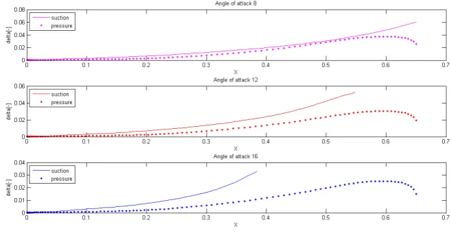
Figure 3.1: Boundary layer thickness extracted from Xfoil simulations

Figure 3.1 shows the plot of boundary layer thickness along the suction and pres-sure side of the airfoil for angle of attack 8, 12 and 16 degrees. The boundary layer thickness is shown only for region of non-separated flow. It can be seen that the separation starts at 12-degree angle of attack at x = 0.55. Based on the boundary

(19)

3.2. LIFT-COEFFICIENT 11

than 1.2 is maintained in the region normal to it. The boundary layer is resolved with

y+ = 1as this gives a good result for separated flows and double precision is used

to avoid round off errors. Four different meshes used for the analysis which are 300 surface points on airfoil with 300 normal points, 500 surface points with 450 normal points, 500 surface points with 600 normal points and 1000 surface points with 1000 normal points.

[image:19.595.137.465.275.444.2]

3.2 Lift-coefficient

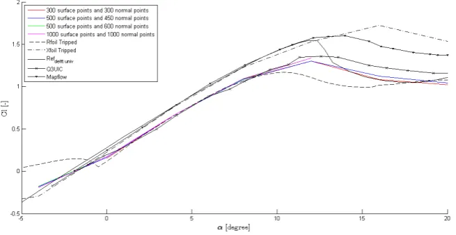
Figure 3.2: Comparison of lift coefficient obtained by various numerical methods and experimental data

The plot of lift coefficient versus Angle of Attack (AoA) is shown in the figure 3.2. The results for the four meshes overlap on each other indicating a grid independent solution. The experimental data and the Mapflow result involves transition and so they predict higher lift coefficient (Cl) values than the corresponding AoA from other

numerical tools. The Cl from SU2 are comparatively lower than non-tripped cases

but stalls at around the same position. This is due to the influence of thicker bound-ary layer for turbulent flows where the velocity deficit is large which eventually leads to less difference in freestream and local pressure (δP) and hence lower lift.

(20)

be noted that the performance of SU2 in stall is relatively better than Q3UIC panel method.

[image:20.595.101.450.205.476.2]

3.3 Drag-coefficient

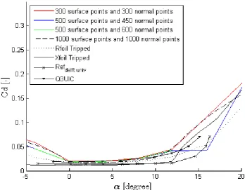
Figure 3.3: Comparison of drag coefficients obtained by various numerical methods and experimental data.

(21)

3.4. PRESSURE COEFFIICENT(Cp) 13

3.4 Pressure coeffiicent (

C

_p

)

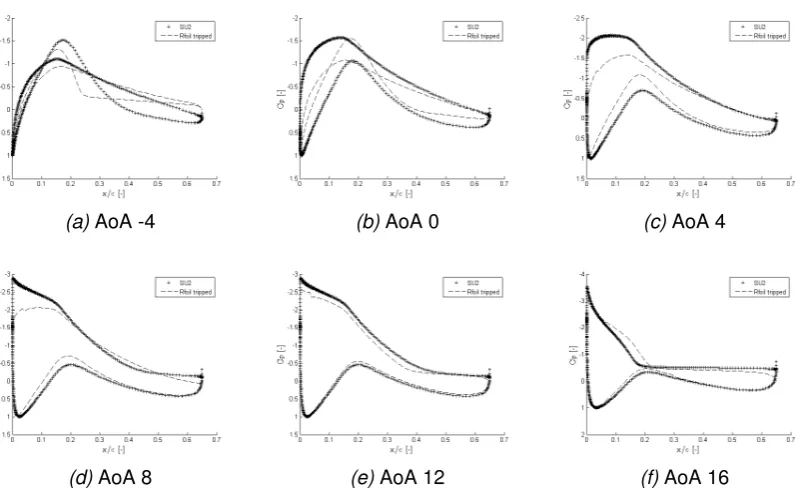
(a)AoA -4 (b)AoA 0 (c)AoA 4

[image:21.595.100.501.130.374.2]

(d)AoA 8 (e)AoA 12 (f)AoA 16

Figure 3.4: Comparison of Cp for the various angle of attacks between SU2 and

Rfoil tripped cases.

Figure 3.4 shows the comparison of the plot ofCp from SU2 with that of the Rfoil

tripped cases for all angle of attacks considered in the polar above. The position of the lowest pressure at the suction side can be seen moving towards the leading edge as the AoA increases. This indicates the increase in the adverse pressure gradient. Also the Cp is over predicted compared to the Rfoil tripped case for all

(22)

(23)

Chapter 4

FFA-W3-301 Airfoil

The airfoil under consideration is FFA-W3-301 which is being used in wind turbines. It has a chord length of 0.6 m with thickness of 30% and it is tested at Reynolds number of 1.6 million in laminar wind tunnel of Stuttgart University. The numerical analysis of airfoil is carried out and compared for fully turbulent flows. Turbulent flows produce more drag compared to laminar flows. However, the flow is stable and the small disturbances are damped out whereas it is not the case with the lam-inar flows. Hence even if the drag is higher for turbulent flows, it is preferred for the reliable performances sacrificing little efficiency. As SU2 is used for turbulent analy-sis, the airfoil experimental data (P. Fuglsang and Madsen [1998]) with leading edge roughness (LER) is taken as a benchmark to compare the results. To obtain LER effect, trip tape is used in experiments. LER is generally observed when dirt is accu-mulated while operating the wind turbine in dirty environment. The SU2 analysis is done at the same Reynolds number of 1.6 million and validated with the experiment and the Navier-Stokes solver Ellipsys 2D for turbulent flow conditions. The Xfoil and Rfoil tripped cases are also considered for comparison. Tripping of Xfoil and Rfoil is done at x/c=0.05 from the leading edge both on pressure side and suction side. The value of x/c for tripping in both Xfoil and Rfoil is chosen in such a way that the stagnation point remains just before the tripping point even at very high angle of attack. Since the airfoil under consideration is very thick, Rfoil tripped scenario is considered a very good benchmark to compare the SU2 results.

4.1 Mesh Generation

2D structured O-mesh is used for the analysis. Structured mesh offers simplicity and easy data access. The element choice is quadrilateral as this is highly efficient to get good convergence and high resolution. The boundary layer is refined with

y+ = 1. The wall spacing s is calculated based on, (Schlichting [1979]) :

(24)

δs=y+ν/ρu∗, (4.1)

where ρ is the density of air, µ is the dynamic viscosity and u∗ is the friction

ve-locity. The density and dynamic viscosity are taken at the conditions of standard temperature and pressure. The friction velocity is given by

u∗ =pτw/ρ,

where, τw = 0.5Cf ∗ρ∗U2,

Cf = 0.0576∗Re−1x /5 f or 5·10

5 _{< Re}

x <107,

(4.2)

with y+ the wall spacing δs is calculated to be8.5·10−6. The wall spacing is given

as the constraint at the boundary layer. The far field is fixed at 90 times the chord length for minimizing the effect of boundary conditions on calculated flow variables. The O-mesh is preferred due to its larger stability at the trailing edge for high gradi-ent flows (Lutton [1989]). This is due to the large accumulation of grid points near the trailing edge which facilitates smooth gradient transformation. The O-mesh also allows better estimation of angle of attack at Clmax. The skewness of the mesh is

kept under 0.67 and the area ratio between the cells around a maximum of 1.4. The aspect ratio which is the ratio of length to width is kept under 4000. The larger val-ues of the above properties than prescribed leads to convergence problem and bad interpretation of the result.

Figure 4.1 shows the mesh generated as per the above mentioned parameter with 300 points on the airfoil surface and 400 points normal to it. On performing simula-tion, it is found that in some points the y+ exceeds 1 even though the wall spacing

(25)

[image:25.595.101.501.172.620.2]

4.1. MESHGENERATION 17

(26)

[image:26.595.127.451.133.305.2]

4.2 Finding the right wall spacing:

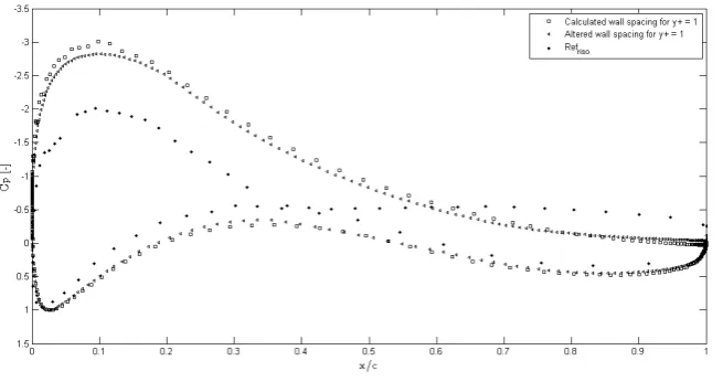
Figure 4.2: y+ for theoretical and altered wall spacing

Figure 4.2 shows the plot of y+ versus dimensionless x-coordinate of the airfoil for the previously shown mesh at 10 degrees angle of attack. The theoretically calculated wall spacing of 8.5·10−6 for y+ = 1 yields y+ value of 1.8 at the suction

side of the airfoil near the leading edge. Even though the calculated wall spacing utilises the local Reynolds number, this higher value ofy+at the leading edge is due

to the high angle of attack which is not taken into account while calculating the wall spacing. In order to get the y+ less than 1 even at higher angle of attack, the wall

spacing is linearly reduced to3.5·10−6 for which they+remains less than 1 around

[image:26.595.124.452.535.708.2]

the entire airfoil as shown in the figure as altered wall spacing.

Figure 4.3: Comparison of Cp for theoretical and altered wall spacing with

(27)

4.3. STEADY ANDUNSTEADY SIMULATION 19

Figure 4.3 shows the plot of pressure coefficient (Cp) versus dimensionless

x-coordinate from the SU2 analysis for the same mesh. This includes the results for calculated and altered wall spacing along with the experimental values for angle of attack of 10 degrees. At this angle of attack the flow begins to separate as evident from the experimental data where the change in pressure coefficient is very little towards the trailing edge beyond x/c = 0.6. Also SU2 predicts the separation but

at a farther position in the chord atx/c = 0.83. At this point the change in pressure

coefficient starts to become insignificant. The separation is almost at the same point for both theoretically calculatedδs and correctedδs. However, for the corrected wall

spacing theCpdistribution lies closer to the experimental value. Hence the corrected

wall spacing of3.5·10−6 is utilised in the remaining analysis.

4.3 Steady and Unsteady simulation

Both the steady and unsteady simulations are performed to compare the result with the experimental data. The steady state simulation is based on the method previ-ously described with the choice of turbulence model as SST. Further the unsteady simulation is carried out to check for the improvement of the solution. For the un-steady simulation, dual time stepping is used to achieve faster convergence. Implicit method can also be used which retains higher order of accuracy. This facilitates larger time step without affecting the solution convergence. But the usage of implicit method is expensive for both 2D and 3D cases as it involves large number of points and require huge system of equations to solve. Therefore dual time stepping is pre-ferred.

While solving the Navier-Stokes equations, the momentum equation is uncoupled as velocity and pressure terms and solved separately. The velocity is calculated as an intermediate step followed by the pressure in the next time step. Finally the ve-locity is corrected in 3rd step. This method of solving is1st _{order pressure accurate}

as pressure is completely disintegrated in the equation. This is overcome by includ-ing pressure partially in step 1 while evaluatinclud-ing intermediate velocity. However, 2nd

(28)

4.3.1

1

st

order dual time stepping

Pseudo time stepping has been used in steady state simulations for rapid conver-gence of the solution in a robust way. However, it uses1st order backward temporal

discretisation which is not very good for simulation of unsteady flows.

4.3.2

2

nd

order dual time stepping

The2nd order method is implemented to get2nd order solution for the transient flow.

It consists of two temporal terms: a physical and a global time integration term. The former term is used to fit the physical phenomena under consideration while the later is used to facilitate quicker convergence. The solution of each unsteady time step is like the converged result obtained with the pseudo time step. While implementing dual time stepping, only the diagonal terms of the Jacobian in the steady state need to be changed with the addition of source term from previous time step. However, it has a drawback that it requires to store three different time steps. i.e. the current time step and two past time steps.

(29)

[image:29.595.122.520.88.524.2]

(30)

[image:30.595.105.508.90.523.2]

(31)

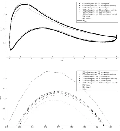
Figures 4.4 and 4.5 show the steady state and unsteady simulations for differ-ent meshes for angle of attack of 6 and 10 degrees respectively. The mesh utilised include 500 points on the airfoil surface and 750 points in the normal direction (i.e. approximately 375000 cells), 1000 points on the airfoil surface and 750 points in the normal direction (i.e. approximately 750000 cells), 1000 points on the airfoil surface and 1000 points in the normal direction (i.e. approximately 1000000 cells). For both cases of 6 and 10 degrees angles of attack the results obtained from all meshes converge to experimental data better than Xfoil tripped case but not as good as that of Rfoil. The results from Rfoil lies closer to the experimental data but still there is an over prediction.

From the figures, it can be seen that the higher the number of cells on the sur-face or the normal direction the better the accuracy of the result as expected. The unsteady simulations provide better results for the corresponding number of cells than that of the steady case. As can be seen from the figures the increase in num-ber of points makes theCp value closer to that of the experiment with the unsteady

case 1000*1000 points reaching the highest accuracy. This seems that as number of cells increases, results that are closer to the experiment could be obtained. For 6 degrees angle of attack where there is no separation, the trend ofCpis similar

to that of the experiment and the result lies closer to Rfoil. However, for 10 degrees angle of attack when there is separation, the result from SU2 is not closer to Rfoil or the experiment. Also the trend is not the same .i.e. SU2 predicts separation at a later point along the chord as evident from the position where the change in Cp

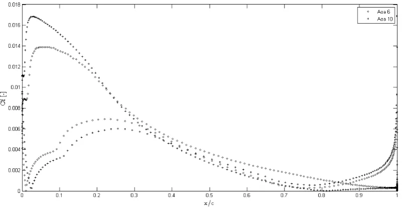
starts to be negligible. Rfoil predicts the separation at x/c=0.6, according to the ex-perimental data the separation is at x/c=0.5 whereas from SU2 it is estimated to be x/c=0.833. The plot ofCf from the result of one of the meshes is shown below which

(32)

[image:32.595.106.508.88.296.2]

Figure 4.6: Cf for Angle of attack of 6 and 10 degrees

Figure 4.6 shows the skin friction coefficient for 6 and 10 degrees angle of attack, with the later indicating the separation at x/c = 0.833. This can be visualised from

the point whereCf reaches zero indicating no shear stress as the flow is separated.

The same can also be visualised from the vorticity plot shown below in figure 4.11 because the flow takes the form of eddies or vortices when the flow separates.

4.4 Polar plot

4.4.1 Choice of the mesh

(33)

[image:33.595.114.521.88.524.2]

4.4. POLAR PLOT 25

(34)

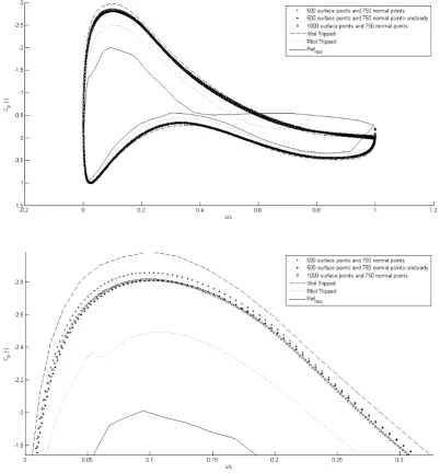
Figures 4.7 show the plot for 6 degrees and 10-degree angle of attack for differ-ent meshes with 300, 400, 500 points on airfoil surface and varying the points in the normal direction. For both 6 and 10 degreesCp follows the same trend as discussed

in the previous section. The mesh with 300 points on the airfoil surface and 400 points in the normal direction seem to give better prediction at 10 degrees which is the beginning of the stall region. Also the choice of 120000 cells mesh is made by keeping in mind that the same mesh will be used for 3D simulation where additional points needs to be added in 3rd dimension which increases computational cost. As described before in section 4.2, the solution converges better if the y+remains

less than 1. For the chosen mesh, the wall spacing is kept as3.5·10−6(which is the

altered value as in section 4.2 ) and they+obtained for all angle of attacks is shown

[image:34.595.112.509.316.532.2]

below.

Figure 4.8: y+ for various angle of attacks

Figure 4.8 shows the y+plot versus dimensionless distance of airfoil. It is evident

that with the corrected value of wall spacing they+remains less than 1 even at high

(35)

4.4. POLAR PLOT 27

[image:35.595.122.521.134.341.2]

4.4.2 Polar (Lift-coefficient)

Figure 4.9: Plot of lift coefficient (Cl) versus angle of attack

(36)

[image:36.595.108.511.126.333.2]

4.4.3 Polar (Drag-coefficient)

Figure 4.10: Plot of drag coefficient (Cd) versus angle of attack

Figure 4.10 shows the plot of drag coefficient for the same airfoil. The results from numerical tools under predict the drag value compared to experiment. SU2 results are comparatively under predicted in the entire domain than Ellipsys or Rfoil tripped simulations. In the linear region of unseparated flow, the steady and unsteady flows under predicts to around 30 % in comparison with experimental data. However, in the separated region the under prediction drastically increases to 200 to 300%. SU2 under predicts the drag coefficient to a maximum of 40% and 3% in the linear region in comparison with Ellipsys simulation and Rfoil tripped cases respectively. However, this under prediction decreases to around 25% and increases to 80% respectively in the separated region.

4.4.4 Vorticity

(37)

4.4. POLAR PLOT 29

(a)AoA -4 (b)AoA 0

(c)AoA 4 (d)AoA 8

(e)AoA 10 (f)AoA 12

[image:37.595.86.525.73.698.2]

(g)AoA 16

(38)

[image:38.595.105.508.249.459.2]

Figure 4.11 shows the plot of vorticity contours for angle of attacks -4,0,4,8,10,12 and 16 from top left. From the plot it is clear that the separation begins to happen at angle of attack of 10 degrees. The flow becomes fully separated at 16 degrees as can be seen from the figure. For negative angle of attack at -4 degrees (top left) the flow separates due to the camber of the airfoil. Even though the vorticity gives the clear picture of the flow separation, the exact point of separation can be studied from the skin friction. At this point skin friction eventually become zero as there is no wall shear stress when the flow separates.

Figure 4.12: Skin friction coefficient for various angle of attacks

Figure 4.12 shows the plot of skin friction coefficient (Cf) in the suction side of

the airfoil to indicate the point of separation. The plot uses the result from SU2-fully turbulent, Rfoil tripped and Xfoil tripped cases for angle of attack of -4 till 12. In Rfoil the value of H becomes maximum at the point whereCf reaches minimum. The

re-sults from Rfoil are given for fully tripped flow and the maximum value of H indicates flow separation, where the displacement thickness rapidly increases. In the results from Xfoil and SU2, the separation is marked by the point where Cf becomes zero

(39)

4.5. BOUNDARY LAYER THICKNESS 31

4.5 Boundary layer thickness

The boundary layer is formed at the immediate vicinity of the airfoil where significant viscous effects prevail. For the turbulent flow as in here, the boundary layer contains eddies and swirls and is more stable with larger thickness than laminar boundary layer as larger momentum is imparted into. The boundary layer tends to grow as the result of adverse pressure gradient and velocity reduction in the direction from leading edge to trailing edge. The geometry used for SU2 simulation is resolved in the near wall region with y+=1 as this would give a very good estimation for sep-arated flow. Also the usage of y+=1 would give a very good approximation of the boundary layer thickness. The results from SU2 can be used to calculate boundary layer thickness in three ways namely velocity, vorticity, and total pressure methods (Zafar [2011]).

4.5.1 Velocity method

The boundary layer thickness can be obtained by locating the edge of the boundary layer. It is at the position where the local velocity becomes 99% of the free stream velocity in the direction normal to the airfoil. Generally, the velocity increases in the region of favourable pressure gradient and decreases from the point of lowest pressure till the trailing edge in the suction side of the airfoil. Due to this decrease in the velocity, the position where the velocity becomes 99% ofUinf tends to increase

in the direction towards the trailing edge and so the boundary layer thickness. The value ofCpat the surface of the airfoil from the result of SU2 can be used to calculate

the velocity at the edge of the boundary layer using,

u=Uinf

p

1−Cp . (4.3)

The position where this value of u becomes equal to 99% of freestream velocity gives the boundary layer edge. However, the curvature shape of the airfoil tends to accelerate the flow increasing the velocity. Therefore, this method cannot predict the boundary layer thickness properly.

4.5.2 Total Pressure method

(40)

gives the edge of boundary layer. By this way the entire boundary layer thickness can be calculated in the suction side of the airfoil.

4.5.3 Vorticity method

Vorticity is the measure of rotational effect of the fluid and for two dimensional flow is given by,

w= ∂v ∂x −

∂u

∂y. (4.4)

[image:40.595.110.506.504.722.2]

Inside the boundary layer the velocity gradient is very large and so shear stress de-veloped between different streamlines leads to rotational effect and thus non-zero vorticity. However, outside the boundary layer the velocity remains almost close to the freestream velocity and so the vorticity is close to zero. Therefore, the position closer to airfoil in the normal direction where the vorticity becomes zero gives a point of the boundary layer edge. When this is calculated along the entire suction side of the airfoil the boundary layer thickness can be obtained.

(41)

[image:41.595.123.518.85.299.2]

Figure 4.14: Boundary layer thickness for AoA of 4 degrees for FFA-W3-301 airfoil

[image:41.595.123.521.485.719.2]

(42)

[image:42.595.108.506.86.296.2]

Figure 4.16: Boundary layer thickness for AoA of 12 degrees for FFA-W3-301 airfoil Figure 4.13 to 4.16 give the plot of boundary layer thickness calculated from vorticity method, Total pressure method, Rfoil tripped and Xfoil tripped cases for angle of attack of 0,4,8 and 12 degrees in the suction side of the airfoil. In Xfoil and Rfoil the boundary layer is calculated from the correlation,

H1 = 3.15 + 1.72/(H−1),

H =δ∗/θ,

δ=θ.H1 +δ∗,

(4.5)

where δ is the boundary layer thickness, δ∗ is the displacement thickness and θ is

the momentum thickness

As can be seen the boundary layer thickness increases as AoA increases. Xfoil predicts larger boundary layer thickness for all AoA. Rfoil gives boundary layer thick-ness smaller than Xfoil but larger than the two methods from SU2. As the Rfoil is successfully tested for many thick airfoils previously this can be used as the stan-dard for comparison. The boundary layer thickness from vorticity method is obtained by tuning the vorticity (ω) between 0.1 and 0.01 and this method gives the largest

(43)

At 12 degree AoA, the boundary layer thickens drastically at the point of separa-tion and then goes off from the surface due to the complete loss of skin fricsepara-tion coefficient (wall shear stress). This behaviour is predicted by Rfoil beyondx/c = 0.4

(44)

4.6 3D simulation

3D simulation is performed on the same airfoil for the mesh of 120000 (300*400) points in 2D. This mesh is extruded with 17.5 mm thickness including 60 points in the lateral direction which leads to 7.2 million cells in total for 3D mesh. The 3D sim-ulations for AoA of 6 and 10 degrees are performed andCp along the dimensionless

[image:44.595.107.468.222.623.2]

distance over the airfoil are plotted below.

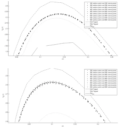
Figure 4.17:Cp for angle of attack of 6 and 10 degrees for 3D and 2D cases/

The figure in the top shows the Cp for AOA of 6 degrees and the one on the

bottom is for AoA 10 degrees along with experiment, Rfoil and Xfoil tripped results. The 2D plot shows theCp for 3D along the length of the chosen span and so multiple

values of Cp can be visualised on the same position. Rfoil results lies closer to the

(45)

4.6. 3D SIMULATION 37

(46)

(47)

Chapter 5

Conclusions

The compressible flow solver, SU2, performance for incompressible flows is studied with two different airfoils namely FFAW3301 and DU97W301. It is found that the lift coefficient is over predicted and the drag coefficient is under predicted than Rfoil and experimental data. The percentage of variation in prediction differs in the linear and the stalled region for both the lift and drag coefficients. The results from the two airfoils depict that the lift coefficient are over predicted to a maximum of 9 % and 5% than the experiment and Rfoil respectively in the linear region. However, in the stalled region the over prediction increases to around 30 to 35% and 15 to 20% respectively. At very high angle of attack say 20 degrees, the Cl over prediction is

reduced to 4 to 7% in comparison with Rfoil. On the other hand, the drag coefficient from SU2 is under predicted to around 15 to 20 % as compared with Rfoil in the linear region and to more than 100% in stalled region. The preliminary 3D results lie in close proximity to Rfoil and so more accurate than 2D results. However, this is acheived at the expense of the computional cost. Furthermore, the usage of theoretically calculated wall spacing makesy+>1in region closer to leading edge

at high angle of attack. This also affects the accuracy of the results. So the wall spacing need to be reduced to around half of the calculated value to maintain y+

less than one at all positions around airfoil and to get accurate results. Finally, it is found that the SU2 predicts separation exactly at the same angle of attack as that of experiment and Rfoil. However, the point of separation is predicted at a later position in the suction side of the airfoil surface than that of experiment and Rfoil. The results from SU2 looks satisfactory with small deviation in the region of non-separated flow. Its performance still need to be improved in the stalled region.

(48)

(49)

Bibliography

A. K. Lonkar T. W. Lukaczyk D. E. Manosalvas K. R. Naik A. S. Padron B. Tracey A. Variyar A. C. Aranake, S. R. Copeland and J. Alonso. Stanford University Unstructured (SU2): Open-source Analysis and Design Technology for Turbu-lent Flows. AIAA Journal, 51(January):1–19, 2014. ISSN 0001-1452. doi: 10.2514/1.C032491.

K. S. Breuer J. W. M. Bush C. Clanet M. Fermigier S. Hochgreb J. R. Koseff B. R. Munson K. G. Powell D. Quere J. J. Riley C. R. Robertson A. J. Smits S. T. Thoroddsen J. M. Wallace G. M. Homsy, H. Aref. Multimedia Fluid Mechanics.

Cambridge University Press.

H. Ozdemir G. Ramanujam and H. W. M. Hoeijmakers. Improving Airfoil Drag Predic-tion. 34th Wind Energy Symposium, (January):1–12, 2016. ISSN 2016-0748. doi: 10.2514/6.2016-0748. URLhttp://arc.aiaa.org/doi/10.2514/6.2016-0748.

K. Gersten H. Schlichting. Boundary layer theory. Mc Graw Hill, eighth edition,

2000.

C. Kong. Comparison of Approximate Riemann Solvers. Thesis, (May):1–69, 2011.

URLhttp://wap.rdg.ac.uk/web/FILES/maths/CKong-riemann.pdf.

M. J. Lutton. Comparison of C-and O-Grid Generation Methods Using a NACA 0012 Airfoil. pages 1–129, 1989. URL http://oai.dtic.mil/oai/oai?verb= getRecord{&}metadataPrefix=html{&}identifier=ADA216375.

M. Manolesos and J. Prospathopoulos. CFD and experimental database of flow devices, comparison. Avatar Task 3.1 Report, (February):1–106, 2015.

K. S. Dahl P. Fuglsang, I. Antoniou and H. Madsen. Wind tunnel tests of the FFA-W3-241, FFA-W3-301 and NACA 63-430 airfoils, volume 1041. 1998. ISBN

8755023770.

H. Schlichting. Boundary Layer Theory. Mc Graw Hill, 1979.

I. Zafar. Numerical Investigation of Boundary Layer Characteristics for Transitional Flow over 2D Airfoils. Thesis, (October):1–102, 2011.

CFD analysis of 2D and 3D airfoils using open source solver SU2