Visualization and analysis of vortex propagation from a jet pump

(1)

Bachelor of Science

Visualization and Analysis of Vortex

Propagation from a Jet Pump

Author: Koen_{’t Hart}

Supervisor: Ir. J.P._Oosterhuis

Chairperson:

Prof. Dr. Ir. T.H._{van der Meer}

External Examiner: dr. H.K._Hemmes

A thesis submitted in fulfilment of the requirements for the degree of Bachelor of Science

at the

Research Group of Thermal Engineering

in the

Department of Engineering Technology

(2)

UNIVERSITY OF TWENTE

Abstract

Faculty CTW

Department of Engineering Technology

Bachelor of Science

Visualization and Analysis of Vortex Propagation from a Jet Pump

by Koen’t Hart

Traveling wave thermoacoustic engines lose efficiency due to Gedeon streaming. If a

jet pump is applied to the engine it counteracts the streaming by suppressing the

time-averaged mass flux through the closed loop of the engine. Placing the jet pump inside the

engine creates certain flow field effects due to “minor losses”.These flow field effects are

oscillatory and have not been qualitatively recorded. The set-up used at the University

of Twente to create acoustic sound waves allows flow visualization of the flow field

generated by the jet pump. A high speed camera records smoke inserted with a smoke

wire.

Vortices are found in the recorded images, and the purpose of this research is to create an

algorithm to trace these vortices as they propagate through the flow field. The algorithm

also calculates the speed with which they propagate but this is not the main focus. The

created algorithm is analyzed using ROC-curves to determine if the algorithm is

bene-ficial for the detection of vortices. The algorithm needs the input of some variables to

allow proper detection, the influence of these variables is documented. There is a relation

between the frequency of the acoustic sound wave and the size, speed and propagating

distance of vortices. The variables therefore need adjusting for the vortices of higher

acoustic sound waves. The development of the algorithm showed the potential of using

these algorithms in the analysis of the other flow field effects. Further improvements are

(3)

Acknowledgements

To start I would like to thank Joris Oosterhuis for the supervision during this bachelors

assignment. Thanks to his quick acceptance I was able to do this assignment on such

short notice. His help, guidance and great feedback contributed to the quality of this

bachelors assignment. Furthermore the approach of Theo van der Meer with the weekly

monday morning meeting created a platform for open discussion, encouragement and

creativity. These meetings would be pointless though without the contribution of the

participating members: Simon, Citra and Rob. I want to thank Citra personally too,

for allowing me to help with her master thesisn, through which I quickly got familiar in

the set-up and the theory of thermoacoustics. Joost also deserves some recognition for

putting me in touch with Joris.

Thanks also go out to my friends(especially Mateo for lunching and working hard with

me every day, and Jorrit for providing dinner), my girlfriend Bella, parents Edith and

Erik, sister Robin and the rest of my family for their unending support and always

present love.

(4)

Introduction

This research aims to study the flow field near a jet pump in a thermoacoustic setup.

The study focuses on registering vortices propagating from the jet pump, in images

recorded with a high speed camera, with Matlab software. The expected results consist

of an algorithm which tracks the propagating vortices for a wide range of images with

the required accuracy.

This thesis will give a basic explanation of thermoacoustics, to understand the streaming

effects and thus the reason for researching the jet pump. Furthermore the process

and the experimental setup for image acquisition is described. The final step of the

thesis is showing the post-processing steps and tools considered and applied, ending

with the conclusion on the accuracy of the developed algorithm and possibilities for

future improvements.

1.1 Thermoacoustic Devices

Thermoacoustics, as the name suggests, consists of two physical phenomena:

Acoustics is the science of all mechanical waves (i.e. vibration, sound, ultrasound and infrasound) in a particular medium (i.e. gasses, solids and liquids).

Thermodynamics is the transfer of energy from location with a high temperature to location with a low temperature.

This interaction is called thermoacoustics, wherein a generated temperature difference

is used to create sound waves and vice versa. A device using thermoacoustic

princi-ples is called a thermoacoustic device. These devices use acoustic waves, in a channel

where a temperature gradient is present, to cause thermal expansion and contraction.

(7)

Chapter 1. Introduction 2

If these are traveling waves, the thermoacoustic device is theoretically able to achieve a

Stirling efficiency[2]. An example of such a device is the Los Alamos National Laboratory (LANL) thermoacoustic traveling wave engine shown in Figure 1.1. This particular engine has been a reference for many studies including this thesis.

1.1.1 A Brief History

Figure 1.1: the Los Alamos National Laboraty researched

engine[2]. To get a better understanding of thermoacoustic

de-vices it is necessary to have a background in its

his-tory. Thermoacoustic effects have been noticed many

years ago. For instance, glassblowers experienced

sound generation by heating a closed-end tube. This

became known as the Sondhauss effect in 1850[9]. Air is heated at the closed end, and this

consequen-tially increases the pressure. The air then flows to

the cool open end, transferring heat to the wall of

the tube until it briefly compresses a small part of

the atmosphere. This creates a propagating sound

wave. Shortly after this compression, the atmosphere

pushes air back into the tube to repeat the cycle. The

Dutch professor P.L. Rijke invented a similar tube in

1859 but this particular variant requires a steady flow

of air with two open ends[8].

In 1877 it was John William Strutt, known as the 3rd Baron of Rayleigh, who wrote a book on sound waves

and researched the Rijke and Sondhauss tubes. Lord

Rayleigh wrote down the qualitative explanations for the effects and defined a criterion

for thermoacoustic effects as:

Lord Rayleigh - “If heat be given to the air at the moment of greatest

conden-sation or taken from it at the moment of greatest rarefaction, the vibration

is encouraged”[28]

This is a criterion for a heat-driven oscillation. Rayleigh basically states that if heat is

given or removed at either the highest or lowest density, oscillations are more likely to

happen. He described a relation between heat-injection and density variation.

After Lord Rayleigh’s discovery, research continued on the Sondhauss tube, the Rijke

(8)

cryogenic temperatures. Scientists like Lord Rayleigh, Kirchoff and Kramers created

a formal theoretical study of thermoacoustics but it was not until 1969 with Rott’s

breakthrough in modeling thermoacoustic phenomena that major progress was made[30].

N. Rott described acoustic oscillations for gas in a channel with an axial temperature

gradient, where its dimensions were out of proportion with the sound wavelength. The

lateral channel dimensions were in the order of the gas thermal penetration depth δk.

Penetration depth is the thickness of the layer of gas where heat can diffuse in oscillations,

typically in the order of 1mm. That is much shorter than the acoustic wavelength, which

is typically 1m for thermoacoustic cases. Rott’s linear theory has been verified and found

quantitatively accurate on multiple tests[43].

After this, thermoacoustics has become an important chapter in heat pumps (transfer of

heat by applying work) and prime movers (generation of work by applying heat gradient).

A similar research has been done by G.W. Swift and many others, but it was Swift who

implemented Rott’s theory to create thermoacoustic devices[31]. It was Backhaus with the contribution of Swift who invented the thermoacoustic engine in Figure1.1in 1999. This engine has been constructed by limiting the number of moving parts as motivation,

a topic where many researchers are working on[27][35][5][6][42]. The engine’s main part is the regenerator, with a hot and a cold heat exchanger, which creates the temperature

gradient needed for the conversion of heat to acoustic power. The lack of moving parts

proved to be a challenge, it introduced many side affects which lowered the efficiency

drastically[2]. One of these side effects is acoustic streaming, a mean mass flux through the torus of the engine.

1.1.2 Acoustic Streaming

Rayleigh started researching acoustic streaming more then a century ago. However, some

effects are still not entirely understood. Acoustic streaming is a net mean flow across

the acoustic system. This flow is the result of the generated sound waves, but it is not a

linear effect. This makes analysis with linear acoustic theory impossible. There is more

than one type of acoustic streaming with different characteristics but the common effect

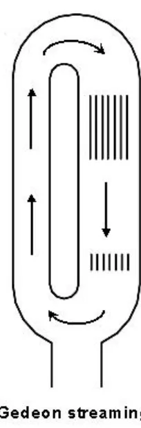
is efficiency loss. In a looped geometry like the Backhaus and Swift engine, Gedeon

streaming can occur. This can be prevented when a jet pump is added.

1.1.2.1 Gedeon Streaming

This type of streaming is based on a net mean mass flow typical for traveling wave

(9)

acoustic velocity and density. Gedeon streaming is relevant for oscillatory

thermoacous-tic engines, and an example of the effect can be seen in Figure1.2. Gedeon assumed the pressure drop, ∆P, linear with velocity U. With that assumption, Gedeon proved that

to have mean mass flow, it is necessary for the flow to fulfill a condition. The flow needs a

resistance in its path which can be seen as an asymmetrical return path to build up

pres-sure. These conditions can be fulfilled through device geometry, density, pressure and/or

[image:9.596.131.233.227.537.2]

temperature variation[4].

Figure 1.2: An example of Gedeon streaming in a torus[31].

It is essential for the performance of a

thermoa-coustic engine to achieve complete elimination of

Gedeon streaming. Gedeon streaming leads to a

time-averaged mass flux M˙2 inside the torus shape

of the thermoacoustic engine[4]. This torus allows the mass flux to return via an asymmetrical path.

Equation1.1 is for time-averaged mass flux.

˙ M2 =

Re[ρ1U˜1]

2 +ρmU2,0 (1.1) Where U2,0 is the second order time-independent

volumetric velocity[2]. The time-averaged acoustic power flow is written as Re[ρ1U˜1]

2 = W˙ . In a case

where there are no actions taken to impose a U2,0

which cancels the first term, the time-averaged mass

flux would transfer heat from the hot to the cold heat

exchanger. This causes undesirable heat leak and

ef-ficiency loss.

Backhaus and Swift state that a non-zero U2,0 must

flow around the torus to enforce ˙M2= 0. Flow is

gen-erated through pressure difference. Hence we would

need an extra part called the jet pump to apply the

required pressure difference to cancel out the mass flux[32].

1.1.3 Jet Pump

A jet pump is a cylindrical part consistent of two openings and a tapered section

con-necting them. As can be seen in Figure 1.3, the jet pump has asymmetric radii Rb

and Rs,ef f where the flow is allowed to enter. The jet pump constricts flow and forces

it through its two openings of different sizes. This causes a sudden contraction and

(10)

either the big or small opening in the jet pump. Expansion occurs when the flow is

reversed and the opposite happens. This means due the oscillatory motion of the flow,

[image:10.596.179.455.148.288.2]

both expansion and contraction occur.

Figure 1.3: A sliced jet pump where the dotted line represents a symmetrical axis. The dimensions are required to define the geometry of the jet pump[7].

If the cross-sectional area of a pipe gradually decreases, mass conservation requires

an increase in mean velocity and a decrease in pressure according to Bernoulli. The jet

pump makes this transition abruptly which gives rise to flow separation, vortex shedding,

turbulence, and jetting[26]. These dissipative effects are hydrodynamic and cause the Bernoulli equation to be invalid. More so, the abrupt transition generates an extra

pressure drop known as “minor losses”. This pressure drop allows us to generate a U2,0

[image:10.596.241.390.488.604.2]

to control the mean mass fluxM˙2 from Equation1.1.

Figure 1.4: Schematic diagram of a jet pump. With flow going from a large cross-sectionalab to the small cross-sectional ason the left and in reverse on the right.

Figure 1.4shows two different states of flow. Flow is either going from the large cross-sectional ab to the small cross-sectional as or in reverse. This results in a ∆Pjp which

is dependent on the density of the fluid ρ, velocity of the flow U2 and a minor loss coefficient K. This minor loss coefficient is not symmetric so there is a Kexp s,b and

Kcon s,b for contracting and expanding the flow, the sand b are respectively the small

(11)

only valid in steady flow, they also fulfill the “Iguchi Hypothesis”[26]. Iguchi and Ohmi performed extensive measurements showing the results of an orifice placed across the

bottom of a tube. These results can be described as quasi-steady, so we can separate

the directions of flow[16]. That means that the flow in Figure 1.4 can be calculated separately and added later to find a net pressure drop across the system.

This is one of the assumptions made to calculate ∆Pjp defined by the dimensions of

the jet pump. Two other assumption are: stating that we are able to add the “minor

loss” coefficients for both directions of flow and that the velocity in the jet pump U1,jp

is harmonic. Backhaus and Swift made these assumptions to derive Equation 1.2, this equation is used for the design of jet pumps[2].

∆ ¯pjp=

ρ0|U1,jp|2

8as

"

(Kexp s−Kcon s) +

as

ab

2

(Kexp b−Kcon b)

#

(1.2)

ρ0 is the mean density of the fluid flowing through the jet pump. Equation 1.2 is

used to specify the parameters of the jet pump geometry. With this geometry and

computational fluid dynamics software, the jet pump designs are simulated. To validate

these simulations and research suggesting that the assumption of the ”Iguchi hypothesis”

does not hold up for higher taper angles, we want to visualize the flow field near the jet

pump[34]. If the flow field is made visible, the dissipative effects described above should be detected and those effects can be quantitatively analyzed.

1.2 Flow Visualization

Flow visualization is a means to making a flow field visible and allows an analysis of

the flow effects. These effects happen in fluids which are typically translucent, and

therefore the effects remain invisible. If we want to record the images which merit

flow visualization, we need to add an observable foreign material. The motion this

observable material undergoes is representative for the flow effects taking place in the

region of interest(ROI). Meaningful images can also be created with an optical method.

If density changes in the flow field are sufficiently large, light rays will be disturbed when

passing through. This optical disturbance can be recorded using Schlieren photography

and is representative for the flow field. Figure 1.5 and 1.6 are examples of options for both methods. Previous research done in flow visualization methods concluded that the

addition of foreign particles is most suitable for this situation. This is because the density

(12)

[image:12.596.336.504.82.249.2]

[image:12.596.129.296.91.258.2]

Figure 1.5: Schlierenfoto Mach 1-2 gerader Fl¨ugel[39].

Figure 1.6: The instantaneous con-centration field in the far field of a tur-bulent jet. Made with a laser and

for-eign fluid reactive to light[36].

1.2.1 Foreign Materials

The common element for this type of visualizations is the addition of a foreign material.

The chosen material should not disturb the flow. For the same reason, insertion is a

delicate process. The medium flowing through the jet pump is air, thus transparent and

gaseous, that allows for the addition of either smoke or particles.

1.2.1.1 Smoke

Smoke is widely used as a tracer for visualization. Smoke can be used either as a smoke

screen or as smoke lines[21]. Smoke’s natural buoyancy is useful because it allows the smoke to move as one homogeneous tracer only to be disturbed by the flow. There exists

a great variety of smoke types, not limited to combustion products but any gas that is

visible without optical techniques. The optimal smoke would be nontoxic, naturally

buoyant, stable against mixing and well visible[22].

These requirements prove hard for smoke to fulfill. Inherently all smoke is toxic to a

certain degree. Smoke also has the tendency to accumulate and fill the ROI with smoke or

any deposit it might generate. Flow visualization with smoke is a consideration between

visibility; its susceptibility to disturbance, accumulation and the injection method.

1.2.1.2 Particles

Another option is to add numerous tracer particles to the air flow, these particles are

(13)

response time to the air flow and the quantity of scattered light. The concentration

of injected particles depends on the used technique. Laser Doppler velocimetry uses a

lower concentration, such a concentration that individual particle tracking is possible

between images. This allows the technique to measure particle speed at specified points

inside the ROI[21]. Another technique, particle image velocimetry (PIV), uses a higher concentration so that particle tracking between images is not certain anymore. This

technique uses a laser, a camera and a synchronizer. By illuminating the particles with

a laser sheet a 2D representation of the velocity is made. The particles are illuminated

for a short time, just for two laser pulses. This results in two images which can be cross

correlated to calculate vorticity and velocity. If the images are recorded in stereoscopy

which involves two cameras, PIV can also record a 3D representation of the flow field.

Drawbacks of PIV are the particles involved. The particle’s density will inhibit them

from following the flow field’s motion. The density has to match up with the fluid,

otherwise the natural buoyancy is not present. If the density of the particles cannot be

changed, there is the option to change the density of the fluid. Changing the fluid results

in a change in Reynolds number. Changing the Reynolds number for an experiment

comes with a change in fluid velocity or the object of interest’s size. Also with the use

of multiple cameras, lasers and the particles there are cost and safety concerns.

Therefore the choice is made to visualize the flow with smoke. This method is cheap and

easily reproducible with a constant performance. The drawbacks of smoke are solved by

adjusting the duration of injection or by geometric changes to the set-up. This proves

(14)

Chapter 2

Method

2.1 Experimental Set-up

In this section, the experimental set-up is briefly explained. 1.

Originally constructed at the TU Eindhoven[1], the set-up is re-purposed by the Ther-mal Engineering research group at University of Twente to perform measurements in

thermoacoustics. The set-up consists of three main parts: a loudspeaker, a cone and the

resonator section showed in figure2.1. The loudspeaker creates an acoustic wave which is amplified by the contraction of the diameter from cone to resonator. The resonator

can be modified to fit different purposes. For flow field visualization a test section is

placed. The jet pump, as well as the smoke injection system, can be mounted inside

this test section[34][7]. The test section is a clear acrylic (PMMA) glass tube to allow flow visualization recording. The PMMA material is cheaper to manufacture and is a

1_{The full explanation of specifics about the set-up can be found in the thesis of D. van der Gun[}₁₂_]

Figure 2.1: A schematic drawing of the experimental set-up used throughout the experiments[21].

(15)

Chapter 2. Method 10

lot less fragile than glass. However, the downside of using a cylindrical shape are the

reflections of the light. The jet pump test section is showed in Figure 2.2.

The ending of the resonator tube, also called the termination, can be varied. The

termination is: closed, opened or configured with a resonator. This resonator

simu-lates a traveling wave going through the test section and works for a pre-determined

frequency[34]. The visualizations for this thesis are done with the open configuration.

Figure 2.2: A model of the jet pump test section as designed by F. Dixhoorn[7].

In the test section the different designs of the jet pump can be mounted. The high speed

camera and the smoke wire are not shown. Both specifics will be elaborated in Chapter

2.2.

2.2 Image Acquisition

The following chapter describes the process of acquiring the images of the flow. This

involves all actions to obtain qualitative images. Choices are to be made to obtain

the images. In the following chapter these choices will be discussed and in the end a

summary will conclude the choices made in the visualization of flow for this thesis.

2.2.1 Light

Light is required to capture the images. This light is supplied by a LED light source

shown in Figure 2.4. The PMMA tube is highly reflective, making the placement of the LED light source critical. Multiple different light locations were tested. The final

choice of the test section set-up is shown in Figure 2.3. To minimize the reflections, it was decided to illuminate the tube from the open end of the resonator. The inside of

(16)

Figure 2.3: A schematice drawing of the test section setup with cam-era and light for standing wave flow

visualization[34].

Figure 2.4: The LED light used to light up the set-up.

the jet pump is designed to function inside of a traveling wave thermoacoustic engine

as described in Chapter 1. Therefore flow visualization with the open termination will increase understanding in the flow patterns of the “minor losses” but it will not be a true

representation. Also this Tests are done with a jet pump with a black face, although

this decreases reflections it also decreases the light inside the tube drastically. This is

important because getting enough light in the tube improves the contrast of the image

and reduces noise.

2.2.2 Camera Setup

These flow effects are high speed oscillatory effects and cannot be seen by the human

eye. The frequencies of the oscillations are between 28Hz and 169Hz. The high speed

camera available is capable of shooting up to 1000 frames per second (fps) with the

limited light in the test section. The camera is a Phantom v7.3 high-speed camera with

a Nikkor 40mm lens at aperture f/3.6.

Camera Triggering A control software is used in operating the Phantom high speed

camera. Within this software, it is possible to control all parameters of the camera. It

shows a preview of what is to be recorded and allows for advanced image processing.

With the software the camera is also triggered.

Image Extraction The images are recorded inside the internal memory of the

cam-era. Its internal memory allows recording 8800 frames. The control software can save

these images in multiple formats and is not limited to just video. To import these

(17)

DNG images are digital negatives, an open standard RAW file developed by Adobe, and

accessible by numerous programs including Matlab while retaining their raw file quality.

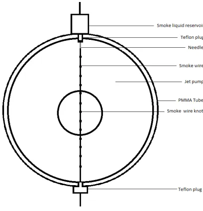
2.2.3 Smoke Injection

A smoke wire is used for smoke insertion. A heating wire is vertically placed inside the

tube and a smoke liquid steadily flows down while evaporating and generating smoke,

shown in Figure 2.5. The amount of smoke generated depends on the material of the smoke wire, smoke liquid, the liquid flow speed and the temperature of the wire. The

material chosen for the smoke wire is based on its strength, its temperature when current

is applied and its diameter. An NiCr 8020 material is chosen with a diameter of 0.2 mm

because of its flexibility and the range of temperatures it can withstand[34]. The wire is mounted between two Teflon plugs, that keep the smoke from leaving the PMMA tube,

prevent smoke liquid flowing along the sides of the tube but more importantly keep the

PMMA tube from melting. The upper plug consists of a reservoir which contains the

smoke liquid and a needle to apply it to the smoke wire. The liquid flows through the

[image:17.596.239.443.394.606.2]

needle along the smoke wire.

Figure 2.5: A schematic drawing of the smoke wire applied to the test section.

When this flows too quick there is minimal evaporation of smoke liquid, hence resulting

in minimal smoke generation. This is solved by increasing the hindrance to flow of the

smoke liquid along the wire by tying knots which hold small amounts of oil to evaporate.

The knots are spaced 1 cm apart across the full length of the smoke wire to produce a

(18)

[image:18.596.192.443.88.399.2]

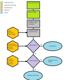
Figure 2.6: A flow chart showing the flow visualization process.

2.3 Image Post-Processing

There are almost 9000 images captured with each flow visualization and these images

re-quire analysis. The analysis is focused on vortex detection. Manually doing this involves

measuring pixel distance between vortices in subsequent frames. This is meticulous and

exhaustive work which is also prone to user induced errors. For these reasons, it is

pre-ferred to create an automated algorithm in Matlab which requires minimum user input

to detect the vortices and save their paths, a flow chart of the flow visualization is shown

in Figure 2.6. In the following section, the process of post-processing is discussed.

2.3.1 Vortex Detection Algorithm

The suggested algorithm needs to locate, track and measure the vortices leaving the jet

pump. This algorithm, would ideally be fully automated, where importing the images is

the only manual task. Realistically, it still requires parameters from the user to produce

(19)

[image:19.596.182.452.81.282.2]

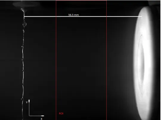
Figure 2.7: A schematic drawing showing the scale and the region of interest.

is a heavily researched subject and this provides many worked-out options with easy

implementation.

2.3.1.1 Loading Images, Conversion and Mean Image subtraction

The selected frames go through multiple steps to create gray-scale images. The images

are balanced. Balancing changes the distribution of the image data created by the

camera sensor. The images then undergo a demosaicing process, this aims to create the

true pixel values from the RGB values created by the Bayer image sensor in the high

speed camera. The remaining step is changing the image into a gray-scale, the result

is a matrix of 800×600. The length scale is determined from a sample image. The

length between the nozzle of the needle and the jet pump is taking as a reference. In

Figure 2.7 the length is shown and the scale derived from it is 0.0495 mm

pixel From the range of images loaded into Matlab, a mean image is taken. In this image all steady and

consistent image content is present. This is assumed as the background of the image.

If this background is subtracted, it leaves the foreground for further image processing.

This is called foreground detection and is widely used to detect moving objects from

static camera images. This background serves as a reference frame when subtracted.

This results in higher contrast of motion between subsequent frames.

2.3.1.2 Cropping, Filtering and Normalizing

The image is cropped to focus on the region of interest(ROI). The region is shown in

(20)

acoustic wave creating the vortices, the Y-axis is fully selected to be sure to capture the

vortices. This is further elaborated in Section2.4.1.1.

This cropped image is then filtered. Filtering is done to reduce the noise introduced by

the low light situation. There are 3 filters implemented in the algorithm. These filters

are chosen for their renown in image noise reduction. The following filters aim to reduce

noise but remain detailed on the edges of objects. To get the desired effect of a filter

it needs the input of a filter window size and a variance called standard deviation σ.

Filters are applied by multiplication in the form of Equation2.1.

IB =FG,W ×IA (2.1)

FG,W is the applied filter where G is a Gauss filter and W is a Wiener filter. IA,B are

the images on which the filters are applied. The median filter cannot be included here

because it uses a nonlinear method.

Gaussian Filter Is considered as the optimal linear smoothing filter. The negative contribution of frequency components in images is reduced in a controlled manner. the

software implementation of the Gaussian filter uses Equation 2.2.

FG(x, y) =e

− x2+y2 2σ2 (2.2)

The coefficients of the image FG(x, y) are calculated with the help of Equation 2.2, the

coefficients are based on the center of the image. The center size is determined with the

window size and standard deviation σ input[24]. X and y are the distances from the origin in respectively horizontal and vertical direction.

Wiener Filter This linear filter tries to improve images heavily degraded by noise.

It aims to restore the original image by applying a filter. The action of the filter is

deter-mined by the error between the image with corrupting noise and the filtered image[37]. In Equation 2.1the application of the filter is shown, the error with respect to timetis shown in Equation2.3.

e(t) =IA(t+α)−IB(t) (2.3)

Theα term is the delay introduced by applying the filter, in the case of Wiener filtering

α= 0. The filtered image can also be written as Equation 2.4.

IB(t) =

∞

Z

−∞

(21)

The error is squared and then minimized to find an optimal FW(t). This is done by

solving the Wiener and Hopf equation which goes beyond the scope of this thesis[37].

Median Filter This kind of filtering is nonlinear and used for noise reduction. It is based on creating a median value of am×nmatrix. the median value is thus a result

of the values from the neighboring values. The pattern of neighbors is called a window

and these windows can take complex shapes for 2D median filtering. The results are

a filter that has demonstrated the capability to reduce noise whilst retaining feature

boundaries. Matlab implements the filter using the same method. The application of

the filter could cause distorted edges as them×nmatrices which cross the edge of the

images are padded with zeros[24]. These zeros cause the median values of these matrices to be off.

The result is a cropped and filtered image. The type of filter chosen is important to

allow better processing in the following steps. Higher filter strength also lowers the

computational load for the edge detection as there is less detail in the edges to be

detected. The optimal filter for the flow visualization is discussed in Section2.4.1.1.

To make the image values more convenient in mathematical operations and plotting, the

images are normalized. The images are in 8-bit gray-scale so the values in the image

range anywhere between 256 for total presence (white) and 0 for no presence at all

(black). These are given more intuitive values. The values are scaled to be anywhere

between 0 for black and 1 for white.

2.3.1.3 Edge Detection

The vortices in the range of images need to be segmented from the rest of the image.

The grayscale images the algorithm has created can be converted into binary images

with thresholding. The vortices appear to be darker then the surrounding areas. When

a threshold is applied, an image with the vortex present should be segmented as a black

region with white surroundings. The threshold value needs to be correct: too low and

there is no detection; too high and there is over detection.

Because of the importance of the threshold, multiple methods are investigated. The

following thresholding methods are selected because of their performance on comparable

(22)

Otsu’s algorithm This method is available in Matlab within the “graythresh” func-tion. The algorithm assumes that pixels either belong to the foreground class or

back-ground. The optimal threshold is when the overlap of the histograms from these pixels

is minimal. the separated pixels belong to classes (foreground or background). The

process can also be described as minimizing intra-class variance, which is defined as the

weighted sum of variances of the two classes[10].

Every image has a histogram. The method assumes this histogram is divided into two

by threshold t. From the histogram the probability, ωi(t), of a pixel belonging to the

background class of foreground class is determined for both parts, i, of the histogram.

With the histogram, µi is also calculated, this term is described as the mean between

two classes. the intra-class variance,σ2_b(t), is then calculated with Equation 2.5.

σ_b2(t) =ω1(t)ω2(t)(µ1(t)−µ2(t))2 (2.5)

Finding the maxima from Equation2.5forσ2_b(t) for both parts of the histogram results in the corresponding thresholds. The desired threshold is then the average of these two.

Kittler The Kittler method is developed to create a computationally efficient method

to calculating minimum error thresholding. It works on the assumption that the pixel

grey level values are normally distributed[20] and can be separated for the foreground and background in two gaussian curves. A performance curve is made for correct

clas-sification between the foreground and background called the criterion function.

Figure 2.8: Left: A sample image of a grey square with black background; middle: histogram of the sample image; right: criterion function of the histogram with a clear

internal minimum[20].

The criterion function, shown in Figure 2.8, is a subtle manner of finding the right threshold value. for any threshold the criterion reflects indirectly the overlap between

the histograms of the foreground and background. A smaller overlap leads to better

segmentation between foreground and background. So the threshold value which gives

(23)

Kapur The Kapur method calculates the optimal threshold by optimizing the en-tropies for two different distributions of graylevels. Entropy is a statistical measure for

describing the randomness of graylevels in the image. Minimizing the random gray level

probability will increase the accuracy of the image’s histogram. With the histogram it is

possible to find the threshold which maximizes the segmentation of information between

the foreground and the background[19]

Triangle A method which originated from medical image analysis. The threshold is

geometrically determined from the histrogram of the pixel intensities. The maximum of

the histogram is detected and a line is drawn between this maximum and the highest

level of the histogram (usually 256 in 8-bit images). Now the distance between this

line and the main peak in the histogram is maximized, which gives a location on the

X-axis. In the research performed by G.W. Zack a factor A was added to this to

[image:23.596.216.415.368.539.2]

increase segmentation. In figure 2.9 the geometrical process is shown, the threshold is also indicated[44].

Figure 2.9: The geometrical process of calculating the threshold (THR)[44].

To summarize, the thresholding methods are designed to separate pixels between

fore-ground and backfore-ground. So also between relevant and irrelevant objects. All methods

seem to over estimate the threshold. The threshold constantly gets set too high and to

attain good separation between the images a factor is introduced to reduce the threshold

level. This is undesired, as this increases the user involvement in the algorithm.

Af-ter the threshold is applied, the images are binary. Matlab has built in edge detection

(24)

Implemented in the Matlab algorithm are some basic boundary conditions to simplify

the ROI for the edge detection algorithm. There are three different types of boundary

conditions applied.

Detected regions in the top and bottom pixels of the ROI are removed from further processing. The vortices are propagating from the right to the left in the middle

of the ROI. Any detected regions in the top and bottom are considered pollution.

The left side of the ROI also neglects detected regions but for different reasons. With vortex analysis, in Chapter 2.3.1.4, the propagation speed is calculated but from the preliminary graphs it appeared vortices slowed down near the end. This

effect is not expected and caused by the edge detection algorithm. As the region

moves through the left side of the ROI, it is still detected which results in a lower

detected speed.

The size of the detected region, which has a minimum and a maximum.

2.3.1.4 Vortex Analysis

To improve the accuracy of the found regions and verify if they are vortices, a vortex

analysis is implemented. Verifying the regions is done with more conditions. But these

are specific for the properties of a vortex. The analysis runs through all detected regions

to check if there are any vortices. The conditions state:

Vortices have to propagate to the left. Any regions that is not moving left cannot be a vortex and is deleted. Whether the region is moving left, is determined by

evaluating the location of the center point of the detected region. If this center

point moves left in subsequent frames, the detected regions is consider a vortex.

More detected regions have to follow after the first vortex detection. If a vortex is detected, two other vortices need to be detected in the two subsequent frames.

A vortex can only propagate with a certain speed. To filter outliers from the detected regions a maximum speed of 10 m/s is set and a minimum speed of 0

m/s.

When a detected vortex fulfills these conditions, it is called a trace. These traces are

equal or longer than 3 detections in a row. From these traces the propagation speed is

calculated by differentiating the location of subsequent center points with respect to the

(25)

2.3.2 Alternative Image Analysis Tools

There are many alternative analytically tools to our disposal. The following section will

give a short description of promising techniques capable of correlating two images. The

current Matlab algorithm can detect vortices in frames but does not use any information

available from subsequent frames. This is a highly discussed topic in literature in medical

or surveillance fields of research. These research fields mainly use it to map images on

top of each other using subsequent image information, but that does not mean the

methods can be repurposed to benefit vortex detection and vortex propagation speed

calculations.

2.3.2.1 Image Registration

The following section describes the main algorithm of image correlation. The following

techniques all use this algorithm with only small differences. Image correlation

algo-rithms are used to find correspondences between images. These correspondences can

be found by using multiple techniques with various characteristics. The characteristics

range from landmark positions, contours, surfaces, and volume of intensity plots[17]. The algorithms try to achieve smooth transformation of the geometrically altered image

ZM (often referred to as a moved image) to the reference imageZR. The transformation

is denoted by matrix T(x, y) so that ZM(T(x, y)) is as close to the reference image as

possible[41].

Intensity Based Image Registration For intensity based image registration (IBIR), the geometrical transformationTis created by best matchingZM andZR on their

sim-ilar/dissimilar observed intensities. Applying the transformation matrix to ZM allows

for precision mapping on top of the reference image, establishing a point-by-point

corre-spondence. IBIR can achieve automatic mapping without any prior input about shapes

or features in the reference image. This saves a time consuming and calculation heavy

task for the computer doing the registration.

IBIR can be adapted easily, allowing it to detect vortices based on their generated

intensities, or lack there of. Lets assume frame A contains a vortex, the subsequent frameBalso contains a vortex. The IBIR technique let us match up these vortices and calculate the geometric transformation matrixT. This matrixTcontains the translation

information of the image from where the displacement of the vortex can be derived. This

displacement should be more accurate than with the edge detection method because it

(26)

the highest intesities are centered on each other which generates a more precise center

point of the vortex.

Optimal Mass Preservation Based Image Registration This is similar im-age registration as the IBIR technique but to calculate the transformation matrix T it uses the optimal mass transport theory developed by G. Monge[23] and improved by Kantorovich[18], and known as the Monge-Kantorovich transportation problem[47]. It is a study in the optimization of transportation and allocation of resources. It works

under the assumption of a constant mass during the process of transportation. The

theory behind this goes beyond the scope of this report. Understanding its application

to image registration is however, will be discussed in the following

The same frames are taking as described above,Aand B, and we assume each of them have a positive mass density function µA, B. The assumption that the total amount of

mass per image is the same is made as well. This gives Equation 2.6 for the Jacobian transformation whenu is used to map frameA to frame B.

µA=|Du|µB◦u (2.6)

|Du| is the determinant of the Jacobian of u and ◦ is the composition of functions.

We are now interested in finding a map u which changes the mass preserving mapping

minimally to find the closest match. Here the Kantorovich-Wasserstein penalty L2 is introduced, this places a penalty on the distance the map u has to move each pixel,

weighted by the pixels intensity. This results in a distribution of materials which is

forced to be frame B. This leaves the calculation of the “optimal” map of frame A on

B, this is a heavy computational step but also one with substantial literature research

with multiple strategies to reduce the computational load[46]. With this “optimal” map it is possible to determine the translation of the vortex and use this to calculate is

propagation speed.

Continuous-Field Image-Correlation Continuous-field image-correlation (CFICV)

uses regions instead of pixel intensity values to compare image ZM with image ZR[11].

Simultaneously the transformation matrix T is used to minimize the cost function de-scribed in Equation 2.7

= Z

Ω

[ZMT −ZR]2dΩ→min (2.7)

Ω is the correlation domain. This is the boundary region limited to the size of the image

but commonly split up in smaller regions to increase accuracy. Minimizing the cost

(27)

[image:27.596.242.394.519.615.2]

Figure 2.10: With the continuous-field image-correlation these are the results, from left to right: ZR,ZM andZMT −ZR[11].

In Figure 2.10 we can see examples of the procedure. From the translations of those cubes and its center points we can calculate vectors for velocity and vorticity.

Tracking of Non-Rigid Objects This is not necessarily a method of image

registra-tion but an alternative for edge detecregistra-tion. This technique works by specifying a template

of the object of interest. The process applies a parametric transformation to allow

vari-ability in the template shape. There are promising classical deformable template based

tracking algorithms developed but they function in similar manners[45]. The difference is the assumptions the algorithms make about the object of interest. Assumptions can

be made about the shape, the shape change and to what degree of change[25]. Also the location where the shape is detected can be assumed either anywhere in the image

or a certain region[15]. The algorithms are self learning to a point but still need basic input about the object of interest. In Figure 2.11 an example of non-rigid detection is shown[25]. The final decision on where the object of interest is detected depends on a voting stage, where in this case there were more votes for the right detection.

Figure 2.11: The left images shows the learned shaped and in the right image it shows the detected shape in the larger form. The crosses note the detected places

before voting on which is better matching[25].

The vortex has a particular shape different from the background of the footage. The

shape can be learned or supplied by the user to be implemented into one of the tracking

algorithms. As soon as the vortices are detected and tracked the calculation of the speed

(28)

Salient Motion Object Detection Salient motion means the important or inter-esting motion in recorded footage as opposed to non-salient motion. In the case of

this thesis, the vortices are considered as salient motion while all other movement is

non-salient. Salient motion detection works by performing these steps[40][33]

Step 1 - Calculate the region of change, which is calculated by subtracting subse-quent images and applying a threshold to extract the moving pixels

Step 2 - The optical flow, also known as a 2D motion field, of the pixels is calculated from frame-to-frame.

Step 3 - The direction of the pixel motion inside the region of change is determined. The direction is sorted in X and Y direction.

Step 4 - Pixels which continually move in a constant direction are used as seed pixels. The neighbor pixels are also checked until it grows in a N ×N region of

pixels moving in the same direction. Also described as the salience field.

Step 5 - Objects with salient motion are finally detected when the information form the previous steps is combined.

The result is a salient object, the steps of detecting salient motion can be seen in Figure

[image:28.596.238.394.453.568.2]

2.12.

Figure 2.12: Showing the steps of detecting salient motion. Left top: original image; right top: difference image; left bottom: X-Component of the flow; right bottom: final

detected salient object[33].

The result is a black and white image where with edge detection the object can be

tracked. The tracked regions can undergo vortex propagation speed calculations.

2.3.2.2 Summary

Some of these methods calculate the vortex propagation speed with the same

(29)

the manner of calculating the transformation matrix. After this matrix is found the

algorithm for the vortex tracking would be the same. CFICV method is less useful

for the calculation of vortex speed because it looks in multiple regions spread over the

image and focuses on small changes within those regions. This would make it an

ineffec-tive method for vortex tracing but suitable for displacement velocity calculation. These

methods do have the advantage of tracking regardless of knowing which shape to track

as opposed to the non-rigid object tracking. Therefore this method seems ineffective.

Salient motion tracking seems the most promising method. The vortices move in a

con-stant direction from right to left which is the ideal movement to apply this method. The

implementation in Matlab is not straight forward. It requires an in-depth knowledge

about image/video manipulation and mathematics. However the computational load is

average compared with the other methods. Also taking into account the pixel by pixel

calculations involved in this method.

2.4 Process Validation

The created algorithm manages to track the vortices, plot their paths and calculate

their speeds. However, the accuracy of the acquired data is yet unknown. The following

section gives insight in the accuracy of the algorithm. A method will be introduced for

finding the parameters which dominate the algorithms accuracy.

2.4.1 Statistical Analysis

The algorithms accuracy will be estimated by commonly used methods in statistics.

These methods are often used in image post-processing fields to justify the use of certain

methods. For this reason the statistical tools will be applied on the Matlab algorithms

to justify using it to detect vortices.

A total of 500 images are imported into the algorithm. The investigated parameters are:

filter type, filter strength, threshold method, threshold multiplier, boundary conditions

for edge detection, boundary conditions for vortex detection and region of interest size.

The influence of these parameters is assessed with a ROC-curve, the imported frames

are sampled to find the values required to create these curves.

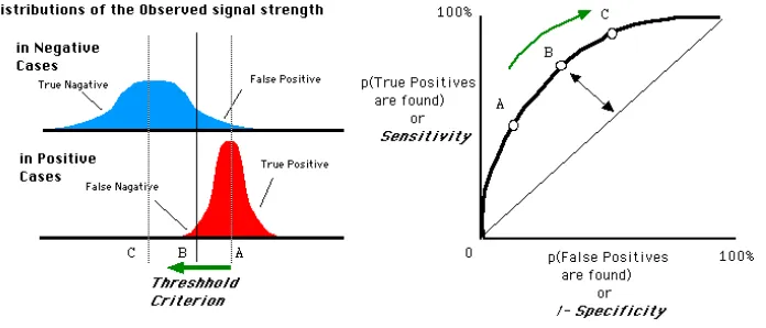
2.4.1.1 Receiver Operating Characteristic Curves

The ROC-curve is used in medical fields to determine whether a patient will need

(30)

Contingency Matrix

Positive Test Outcome

True: False:

Vortex undetected Vortex undetected where a vortex is present where no vortex is

Negative Test Outcome

False: True:

[image:30.596.147.495.310.459.2]

Vortex undetected Vortex undetected where a vortex is present where no vortex is

Table 2.1: Table summarizing the results from the image post-processing in statistical terms.

these decisions. The method compares two Gaussian distributions, one for negative

cases of the algorithm and one for positive cases. The lesser these distributions overlap

the better the separation is between good results and bad results. An example of a

ROC-curve is shown in Figure2.13.

Figure 2.13: An example of a ROC-curve with the distributions for negative and positive cases[38].

On the x axis 1−specificity is denoted, also known as the false positive rate (FPR). This can be written as FPR = FP/(FP+TN), where FP are false positives and TN are

true negatives. They axis is thesensitivityor the true positive rate (TPR). Written as TPR = TP/(TP+FN), where TP are the true positives and FN are the false negatives.

The ideal shape of the ROC-curve would keep close to the left side and only separate

for higher values on the y axis.

The different outcomes of the process, shown in Figure2.6, require reformatting in the terms FP, TP, FN and TN(this is shown in Table2.1).

These outcomes are acquired by sampling the imported images. The images are

manu-ally controlled to see if the detection made the correct conclusions. To get the necessary

accuracy of the outcomes there needs to be a certain amount of sampled images.

(31)

[image:31.596.172.450.87.367.2]

Figure 2.14: An example of a ROC-curve with the threshold data from Othu’s method and the true threshold values for 56Hz frequency.

term from normal distributions. p are the chances for the expected results, p= 50% is

used to give the largest sample size. On the accuracy a margin of error is added, this is

the amount of error tolerable for taking the sample. In the case for the ROC-curves the

desired accuracy is 95% with only 5% deviation.

NSS =NP S

Z2p(1−p) Z2_p₍₁₋_p_{) + (}_N

P S−1)E2

(2.8)

So to achieve that accuracy it is necessary to sample 218 images. So for every plot point

on the ROC-curve 218 images are sampled to find the corresponding TPR and FPR.

ROC-curves are created for the input variables of the vortex tracing algorithm for three

different frequencies(28Hz, 56Hz and 80Hz), shown in Figure 2.6. The vortex decision step will be neglected in the ROC-curve. This decision is made because if a region is

positively detected it could be neglected by the vortex analysis step because it does not

comply with those conditions. If the vortex analysis step would be included this would

change the influence of the variables for the edge detection step. The found variables

might work for the vortex analysis step but are not beneficial for the overall algorithm.

This is due to inconsistency with the decisions for TP, FP, TN and FN. A TP for the

edge detection can be a FP for the vortex analysis if the detection does not comply as

(32)

[image:32.596.168.466.79.310.2]

Figure 2.15: A schematic of the size of the Region of Interest (ROI) which is varied in the x-direction.

In Figure 2.14 a typical ROC-curve is shown. The other ROC-curves are added in AppendixA.

Thresholds In Figure2.14 the effect of the boundary conditions is clearly visible as the decrease in TP comes earlier. The optimal value is different for each frequency but

seems to be significantly higher for higher frequencies. It varies from 0.04 for 28Hz, 0.06

for 56Hz and 0.45 for 80Hz.

Filters From the ROC-curve it becomes clear that Wiener filters are not as effective

as the Gauss filter. This could be explained by the different focus of the filters. The

Wiener filter focuses more on edges between object and the Gauss filter is smoothing of

the whole image. A lower filter standard deviation seems to work better for the lower

frequency acoustic waves.

Region of Interest The ROC-curve shows that if the ROI increases in size, the size of the ROI is varied in the x-direction as shown in Figure2.15, the performance of the lower frequencies is better while the higher frequency performance is less. Higher

frequency acoustic waves create more vortices. When the ROI size is increased, there

start to be more vortices in one frame and this results in faulty center points and thus

(33)

Variable 28Hz 56Hz 80Hz

Threshold 0.75 0.75 0.9

True Threshold 0.04 0.06 0.45

Filter Gaussσ = 5 Gauss σ= 5 Gaussσ= 10

Region of Interest 3 2 1

Boundary Conditions X: 10 X: 10 X: 10

Y: 50 Y: 50 Y: 50

[image:33.596.135.495.79.203.2]

Minimal and Maximal Area Min: 50 Min: 50 Min: 25 Max: 150 Max: 150 Max: 150

Table 2.2: Summary of the optimal values used for the variables to run the vortex detection algorithm.

Boundary Conditions The influence of this variable is inconsequential, the detected points in the ROC-curve are scattered in a small region. When unrealistic values are

chosen though, the performance goes down. This proves that this variable does not

contribute to the algorithm but when the wrong value is chosen it can corrupt results.

The boundary condition on the left side of the ROI was not implemented to increase

the performance of the detection but of the propagation speed.

Minimal and Maximal Area The minimal area proves to be an important variable.

The maximal area influence increases for higher frequencies. While the data points for

the maximal area are calculated the minimal area was kept constant at 502pxwhich can

be seen for the lower frequencies. The minimal area however, proves that using a larger

area is better for lower frequency acoustic wave because the vortices are larger then.

2.4.2 Optimal Input of the Algorithm

From the ROC-curves the optimal settings are deduced for using the algorithm. Table

2.2gives a summary of the values used to create the results in Chapter 3.

2.4.3 Accuracy

The accuracy is related to the FPR and the TPR. A higher TPR means more TP results

which is desired. The opposite is true for the FPR, the optimal algorithm should detect

the least amount of FP. The FPR and TPR for the optimal settings is shown in Table

(34)

28Hz 56Hz 80Hz

TPR 0.7407 0.7159 0.7006

[image:34.596.237.395.81.134.2]

FPR 0.276 0.1385 0.2951

Table 2.3: FPR and TPR of the optimal algorithm settings for three frequencies.

So the accuracy of the algorithm is best for the 56Hz acoustic sound waves. There the

algorithm detects the most vortices combined with the low FPR achieves the goals of

the algorithm. For the other frequencies the FPR is too high, there over 25% of the

detections are FP.

2.4.4 False Positive Rate Problem

When a high frequency acoustic sound wave creates vortices there is the possibility that

two vortices are in the same region of interest (ROI). In a situation where a vortex leaves

the left edge of the ROI and a new vortex enters on the right side, there is no frame

where there are no vortices. This causes problems for the ROC-curves, more precisely

for the false positive rate, Equation 2.9.

F P R= F P

F P + T N (2.9)

In the situation with no frames without vortices, the number of true negatives, T N,

would be zero. So as soon as the algorithm detects its first false positive, F P, the

F P R = 1 and this changes the interpretation of the ROC-curve. This is a special

situation but it applies in any case with few T N and makes the reliability of the

ROC-curve a discussion topic. It would mean that for higher frequencies the results of the

(35)

Chapter 3

Results

In the following chapter the results will be presented. The intermediate steps of the

algorithm will be shown. The steps are compared with the raw image to clearly show

the contribution of each step to the final detection.

This section shows the preparation of the image before thresholding and edge detection

can be applied. Figure3.1shows the foreground detection method, explained in Chapter

2.3.1.1. The right image contains the foreground information. The mean image contains the smoke wire and the jet pump as well as any reflections and other constant contents.

This technique proves to be very useful. The importance of image quality is diminished

due to the efficiency of the foreground detection method. It shows that the algorithm is

capable of creating qualitative images even if there is pollution in the image, as long as

this is constant. Creating a black jet pump or a black background seems less important

as the algorithm is able to remove this from the image.

Due to the low light situation, the created noise was indistinguishable from the smoke

displacement. Noise made analyzing the vortices manually difficult as the edges of the

[image:35.596.113.522.608.708.2]

vortex could not be accurately determined. Noise was battled with the increase of light in

Figure 3.1: The subtraction of a mean image and the result it gives. Left: raw Image of the first frame; Middle: mean image created from a 500 image range; Right:

subtracted image and normalized to show foreground information.

(36)

[image:36.596.169.464.80.227.2]

Chapter 3. Results 31

Figure 3.2: This figure shows the improvement of filtering, cropping and normalizing. Left: raw image, noise is present; Right: mean subtracted, cropped, normalized and

filtered image ready for thresholding.

the set-up, but due to limitation of the light placement, noise was only slightly reduced.

The left image in Figure3.2 shows an average presence of noise.

The image on the right in Figure 3.2 is made after foreground detection, cropping, normalizing and filtering. This is done with a Gauss filter with standard deviation

σ = 5. The image has more contrast than the right image in Figure 3.1because of the normalization and the noise filtered out by smoothing the image. These are all the steps

performed before the algorithm applies thresholding and edge detection.

Figure 3.3: An identical frame before and after the vortex tracing algorithm is ap-plied. Left: frame with vortex present; middle: frame after post-processing steps and thresholding; Right: edge detection finds region, region fulfills boundary conditions and

could be considered a vortex.

To give an indication of the quality of the algorithm, the left image in Figure3.3shows a vortex in the middle of the image. This vortex is tough to spot. The middle image is the

binary image created by thresholding after all the steps above are also performed. The

binary image now shows a clear detection which could be a vortex. The edge detection

creates the image on the right. It creates a contour and marks it with a yellow center

[image:36.596.169.465.429.580.2]

(37)

[image:37.596.115.521.80.235.2]

Figure 3.4: From right to left these are multiple detections put together to be a vortex. The acoustic sound wave is 80Hz and between eacht there is 1/1000s. This

trace is used for further calculations.

This detection is not necessarily a vortex, this has to be determined with the vortex

analysis. Only when this detection fulfills the conditions described in Chapter 2.3.1.4, is it assumed to be a vortex.

A detection which fulfills the conditions to be a vortex is shown in Figure 3.4. The leftmost image shows a purple detection, this is when one of the boundary conditions is

broken, in this case the detection crosses the left side boundary. In the rightmost image

there is a red detection. This detection breaks multiple boundary conditions.

Figure 3.5: A graph with all traces of three detections or more at 80Hz. The x location should be read in reverse as the origin is placed on the left side of the region

of interest.

When a batch of images is analyzed by the algorithm, it creates Figure3.5. There are 500 images analyzed of 80Hz by the algorithm which at 1000 frames per second gives 0.5

seconds worth of footage. Theoretically there should be 40 vortices traced. In reality the

[image:37.596.180.449.459.623.2]

(38)

[image:38.596.195.434.90.288.2]

Figure 3.6: A Bar chart showing the manually calculated vortex speed and the speed calculated by the algorithm.

The propagation speed calculations are shown in Figure 3.6. There seems to be a difference between the propagation speed calculations done manually or done by the

algorithm. The manually calculated speeds are higher for lower frequencies and decreases

when the frequency gets higher. The trend is the same for both calculations methods but

the decrease is more rapid for the manual calculations. The averages for the algorithm

speed calculations are taken from the traces found for the different frequencies.

The results differ vastly per frequency, and are dependent on many variables. Not all

variables are from the algorithm: the lighting, the amount of smoke in the PMMA tube

are equally important for the algorithm to achieve accurate results. The lighting should

be as constant as possible for the threshold method to calculate the value better. If

the smoke is dispersed equally inside the PMMA tube the vortices appear with more

contrast compared to any other distortions in the smoke.

The results are not always accurate and the algorithm has some errors. In figure 3.7

examples of the errors are shown. The errors lead to missed vortices, faulty traces or no

(39)

[image:39.596.110.523.80.366.2]

Figure 3.7: From left to right, the four types of error. Error 1: incorrect detection; Error 2: multiple detections; Error 3: over detection; Error 4: under detection.

Error 1 - Incorrect Detection An incorrect detection is described as a detection which fulfills all boundary conditions but does not contain a vortex. These errors are

recorded as found regions but when the conditions for vortices are applied, the incorrectly

detected regions can be be neglected from further processing. This error happens when

the maximum area is set too large, and the boundaries too small.

Error 2 - Multiple Detections When multiple regions are detected the algorithm is not able to place the center point in the middle for the vortex because it is not able

to determine which it is. The center point is placed in the middle for all found regions.

So the center point is average between found regions. When multiple regions are found

the center point gives invalid data to the vector analysis algorithm. This could cause

non-vortices to be determined as vortices and vice versa.

The second issue with the center point is caused by the shape of the vortex. From this

camera angle the 2D images cause the vortex to be two dark circles and a slightly lighter

grey connecting them. The edge detection therefore sometimes detects two circles, one

of the two circles or both circles connected. This changes the location of the center point

(40)

The misplacing of the center point causes deviation in the calculated propagation speeds.

The propagation speeds are separated in x and y direction. For the propagation speed

in the x direction, the misplacing causes the speed to increase or decrease drastically.

This creates a large standard deviation of the speed and makes these results unusable for

any conclusions. The propagation speed in y direction should be close to zero because

the vortices move left to right with little to no up or downwards motion. The calculated

propagation speeds are spread between 0 m/s and 20 m/s. This seems to be caused by

the second issue of the center point, between subsequent frames the center point can

jump between any detected region of the vortex. The sudden jump gives rise to the

physically improbable propagation speeds.

Multiple regions are found when the threshold is set too high in combination with a

lot of disturbance in the smoke. The region of interest (ROI) is also important because

multiple detections can occur when the ROI is too large for higher frequencies. Then

before one vortex has propagated fully to the left another is already entering from the

right side of the ROI. The solution would be averaging the center point between found

regions which are close to one and another. This would reduce the inaccuracy introduced

by this error.

Error 3 - Over Detection When the threshold is set too high the segmentation between foreground and background decreases. This results in a detection that is too

large. The boundary conditions then cause the detection to be neglected. Over detection

causes missed vortices.

Error 4 - Under Detection This error is caused by the same reasons as error 3. The threshold in this case is too low, so the segmentation between the foreground and

background is not large enough. The regions are then too small to fulfill the boundary