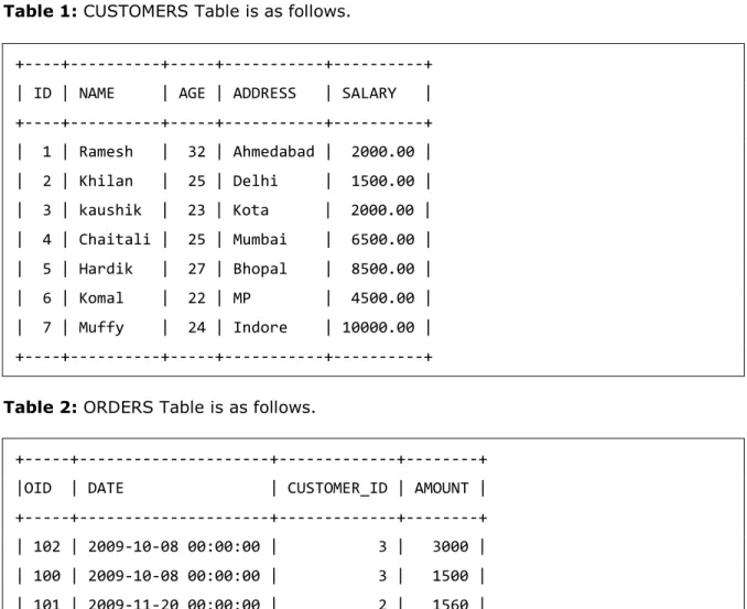
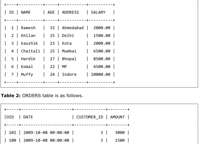
SQL is a database computer language designed for the retrieval and management of data in a relational database. SQL stands for Structured Query Language.
182
0
0
Full text
(2)
(3)
(4)
(5)
(6)
(7)
(8)
(9)
(10)
(11)
(12)
(13)
(14)
(15)
(16)
(17)
(18)
(19)
(20)
(21)
(22)
(23)
(24)
(25)
(26)
(27)
(28)
(29)
(30)
(31)
(32)
(33)
(34)
(35)
(36)
(37)
(38)
(39)
(40)
(41)
(42)
(43)
(44)
(45)
(46)
(47)
(48)
Figure

+7


Related documents
cited here were openly Liberal in politics, they display this liberal consumerism both by promoting poems in praise of consumer goods, written in many instances by the same
of the area.. 4 Yannick Bidel et al. a) Picture of the atom gravimeter on the motion simulator. b) Programmed translation on the motion simulator along the three axes. c)
Database management systems (DBMS) typically use Structured Query Language (SQL) as the interface to access and manage database tables.. The SAS/ACCESS
Investment Justification that addresses each initiative proposed for funding. These Investment Justifications must demonstrate how proposed projects address gaps and deficiencies
For each non-prescribed exception account held by the account-holder and included in the FCS balance use a separate record line and repeat all other data items Account title
nJcoco'roo-Lc,roi-j.doo. iJ4
An adversary, who knows the encryption algorithm and is given the cyphertext, cannot obtain any information about the cleartext (except for its length)..
JALR 23 0x4 Add PCSel clk WBSel MemWrite addr wdata rdata Data Memory we Op2Sel OpCode Bcomp. clk clk addr
