University of Warwick institutional repository: http://go.warwick.ac.uk/wrap
This paper is made available online in accordance with
publisher policies. Please scroll down to view the document
itself. Please refer to the repository record for this item and our
policy information available from the repository home page for
further information.
To see the final version of this paper please visit the publisher’s website.
Access to the published version may require a subscription.
Author(s): WILFRID S. KENDALL AND GIOVANNI MONTANA
Article Title: Small sets and Markov transition densities
Year of publication: 2002
– 371 (revised) –
Small sets and Markov transition densities
by
W.S. Kendall and G. Montana
February 2001
DEPARTMENT OF STATISTICS
Small sets and Markov transition densities
Wilfrid S Kendall
∗and Giovanni Montana
†18th July 2002
Abstract
The theory of general state-space Markov chains can be strongly related to the case of discrete state-space by use of the notion of small sets and associated
minorization conditions. The general theory shows that small sets exist for all
Markov chains on state-spaces with countably generatedσ-algebras, though the minorization provided by the theory concerns small sets of ordernand n-step transition kernels for some unspecifiedn. Partly motivated by the growing impor-tance of small sets for Markov chain Monte Carlo and Coupling from the Past, we show that in general there need be no small sets of ordern= 1even if the kernel is assumed to have a density function (though of course one can taken = 1if the kernel density is continuous). Howevern = 2will suffice for kernels with densities (integral kernels), and in fact small sets of order2abound in the
tech-nical sense that the2-step kernel density can be expressed as a countable sum of nonnegative separable summands based on small sets. This can be exploited to produce a representation using a latent discrete Markov chain; indeed one might say, inside every Markov chain with measurable transition density there is a dis-crete state-space Markov chain struggling to escape. We conclude by discussing complements to these results, including their relevance to Harris-recurrent Markov chains and we relate the counterexample to Tur´an problems for bipartite graphs.
Keywords: COUPLING FROM THE PAST, DATA-MINING, GRAPHICAL MODELS, LA-TENT DISCRETIZATION, MARKOV CHAINMONTECARLO, MINORIZATION CONDI-TION, PSEUDO-SMALL SETS, SMALL SETS, TRANSITION PROBABILITY DENSITY, TURAN PROBLEM, ZARANKIEWICZ PROBLEM.´
AMS Subject Classification: 60J05; 60J22, 65C40
1
Introduction
The notion of a small set was introduced to Markov chain theory by various writers (see for example [18]) and has been exploited to produce a reduction to the discrete case of Markov chain theory for general state-spaces (see Nummelin [17] and Meyn and Tweedie [14] for treatments in book form). The basic idea is to elicit a minorization
condition for a given Markov chain:
∗Supported by EPSRC grant GR/L56831 and EU network ERB-FMRX-CT96-0095.
Corresponding address: Statistics Department, University of Warwick, Coventry CV4 7AL, UK. Email:w.s.kendall@warwick.ac.uk
Definition 1.1 The transition probability kernelK(x,·)satisfies a minorization
con-dition (of ordern) if for some non-vanishing non-negative functiongand some proba-bility measureµwe have
K(n)(x, A) ≥ g(x)µ(A)
for allx, all measurable A. In particular a set C is a small set (of ordern) if its
indicator function can occur together with a constantρ∈(0,1)asg(x) =ρI[C] in a minorization condition of ordern.
The minorization can be used to produce the split-chain construction of Nummelin [16] – see also Athreya and Ney [1] where small sets are used for regeneration argu-ments – and hence to control convergence to equilibrium: as Nummelin wrote, “the ‘elementary’ techniques and constructions based on the notion of regeneration, and common in the study of discrete chains, can now be applied in the general case” [17, page ix]. More recently small sets have been used by Rosenthal [23] to establish rates of convergence for Markov chain Monte Carlo (see also the extended notion of
pseudo-small sets described by Roberts and Rosenthal [20,21]) and also (under the rubric of
gamma-coupling) to produce effective Coupling from the Past (CFTP) constructions in
the work of Murdoch and Green [11,15] (see also some exciting new work on catalytic
perfect simulation by Breyer and Roberts [5,4]).
Closely related to the ideas presented here is the discretization proposed by Robert [19], originally devised for the purposes of Markov chain Monte Carlo convergence assessment. This discretization is based on sub-sampling of a discrete sequence derived from a continuous state-space Markov chain{Xn;n ≥ 0} depending on a sequence
of renewals times, in the following way. Suppose thatXn possesses several disjoint
small setsCi, withi= 1, . . . , Ifor which the minorization condition of Definition1.1
holds with constantsρiand measuresµi. TheCineed not necessarily form a partition
of the whole state-space. Suppose the above splitting construction is applied whenever Xvisits one of theCi. Define the renewal timesτ0= 1andτn, withn≥1by:
τn = inf n
t > τn−1:Xt−1∈Cifor somei∈ {1, ..., I}
and regeneration occurs at timeto
Robert shows that the finite valued sub-sequenceηnobtained fromXtby:
ηn=iifXτn−1∈Ci
is a homogeneous Markov chain defined on the finite state-space{1, . . . , I}.
The theory of general Markov chains assures us of the existence of small sets, but gives no guarantees concerning the order. For the purposes of establishing convergence results this is of no great importance; however order1is required for current CFTP ap-plications. This raises the question, for what sort of Markov chains can one guarantee existence of small sets of order1? As a straightforward exercise in mathematical analy-sis at an advanced undergraduate level, one can show existence for state-space a smooth manifold when the kernel has a continuous densityp(x, y), and indeed then one can show small sets of order 1 abound, in the sense that they can be used to produce a
representation:
p(x, y) =
∞
X
i=1
where thefi(x)are non-negative continuous functions supported on small sets, and the
gi(y)are probability density functions. From this representation one can further deduce
the existence of a latent discrete Markov chain: sinceR
p(x, y)dy = 1it follows that
P
ifi(x) = 1for allx, and sofi(x)may be viewed as a transition probability density
describing transitions from the state-space to a latent countable state-space{1,2, . . .}; and the entire stochastic dynamics of the original chain can be viewed as derived from a discrete state-space chain with transition probability matrix of entries
pij = Z
gi(y)fj(y)dy . (2)
(Finite versions of such constructions, finite-rank Markov chains, are used to derive limit theorems in [25,13]; see also [22].) We continue this line of enquiry in more detail in section§5.
However this particular representation fails hopelessly as soon as we move to the slightly more general category of Markov chains with measurable transition probability densities! Even the obvious step of allowing thefi andgi to be measurable is of no
avail. For, as we show in the next section, there exist transition probability densities for which there are no non-trivial small sets of order1. The construction is based on the construction of a Borel subset of the unit square with no non-null subsets of measurable rectangle form, and is related to a variant of the Tur´an problem from extremal graph theory.
However, and somewhat to our initial surprise, the cause of measurable transition densities is not entirely lost. As we show in section§3, so long as we move to order
2we can construct non-trivial small sets (following known techniques for establishing the existence of small sets), and in fact they abound in the sense that one can build representations of the2-step transition probability densityp(2)(x, y)generalizing that
of Eq. (1), and hence derive an interlacing latent discretization with transition matrix generalizing Eq. (2). Moreover this discretization uses only the measurable structure of the underlying space, rather than its topology: one need only suppose the state-spaceσ-algebra to be countably generated. In Section§4we use the method of§3to show that the weaker notion of pseudo-small sets [20,21] results in the presence of many pseudo-small sets even at order1; however this weaker notion is too weak to allow us to construct latent discretizations. In the concluding section §5 we discuss the latent discretization, and various complements including the extent to which the discretization can be generalized yet again, if one wishes to consider Markov chains whose kernels do not possess transition densities.
Acknowledgements
As well as the financial support noted above, we gratefully acknowledge Gareth Roberts’ suggestion to consider pseudo-small sets, Jeff Rosenthal’s pointer to the literature on finite rank Markov chains, and many other helpful conversations with our Warwick colleagues Saul Jacka, Jim Smith, and Jon Warren.
2
Measurable transition densities may have no
non-null small sets of order
1
exposition, yielding as a first step a probabilistic construction of a measurable subset of[0,1]2which is “rectangle-free”, which is to say, contains no non-null measurable
rectangles. It should be clear to anyone who has studied measure theory that such sets must exist: however we have not been able to find a construction in the literature.
The combinatorial aspect concerns arrays of cells,n×nsquare lattices, the nodes of which are viewed as square cells of sidelength n1, either filled or not, and arranged to pack the unit square. Unions of filled cells form pixellated subsets of[0,1]2. We
will be interested in whether we can find non-negligible filled measurable rectangles: pixellated subsets corresponding to unions of cells of the form
{cell(xi, yj) :i= 1, . . . , r, j = 1, . . . , s}
defined by subsequencesx1, . . . , xrandy1, . . . , yswhererandsamount to substantial
fractions ofn. The basic combinatorial argument constructs random subsets of arrays of cells which have low probability of containing measurable rectangles which are not very small. A Borel-Cantelli argument can then be applied to intersections of the corresponding pixellated subsets, so as to derive the following result.
Theorem 2.1 There exist Borel measurable subsetsE⊂[0,1]2of positive area which are rectangle-free, so that ifA×B ⊆Ethen area(A×B) = 0.
Proof:
Recall Stirling’s asymptotic approximation:
n! ∼ exp
n(logn−1) + 1
2log(2πn)
asn→ ∞. (3)
For fixed rational α ∈ (0,1) we apply Stirling’s approximation to the formula for the mean number of bαnc × bαncfilled measurable rectangles to be found in an n×narray of cells of side-lengthn1, such that cells are filled independently with fill probabilityp. (Herebxcis the greatest integer smaller thanx.) We obtain
mean number of such measurable rectangles =
n
bαnc
2
pbαnc2 ∼
exp n2 α2logp−2n(αlogα+ (1−α) log(1−α)) + log (2πnα(1−α))
(at least fornrunning through the subsequence for whichαnis an integer!). We apply Markov’s inequality to deduce that for fixedε >0andp∈(0,1)
P[ at least onebαnc × bαncfilled measurable rectangle ] ≤
(1 +ε)×exphn2 α2logp
−2n(αlogα+ (1−α) log(1−α)) + log (2πnα(1−α))i (4) for alln≥N =N(ε, α, p)such thatαnis an integer. Clearly the upper bound tends to zero asn → ∞through the relevant subsequence. Moreover the mean area of the corresponding pixellated random set is given byn2p/n2=p.
We now construct a random subsetΞof the unit square[0,1]2as the intersection
of a sequenceHk0,Hk0+1, . . . of such pixellated random sets. The setHkis constructed as the union of filled cells in annk×nkarray of cells of side-lengthn1k, such that cells
are filled independently with fill probabilitypk. We fixε >0and select
α = αk =
1
k p = pk = 1−2−k
n = nk = inf
r >2k∨N(ε, αk, pk) : αris an integer . (5)
The mean area ofΞis bounded below by
E[area(Ξ) ] ≥ 1−
∞
X
k=k0
(1−E[area(Hk) ]) = 1−21−k0,
and thereforeΞhas a positive chance of having positive area (at least ifk0>1).
On the other hand we may apply the first Borel-Cantelli lemma to show that all but finitely many of the events
Rk =
Hkcontains no measurable rectangles of sidelength 1k or greater
must occur. For geometrical arguments show that the failure ofRk forces the
corre-sponding cell array to contain at least onebαnc × bαncfilled measurable rectangle, and by the bound Eq. (4) the failure-probability of this event is therefore bounded above by
constant× 1−2−k
1 2n
2
k/k
2
≤ constant×e−2−k−1n2k/k2 ≤ constant×e−2k−1/k2.
This is summable, and so the first Borel-Cantelli lemma applies.
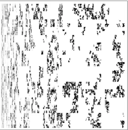
It follows that almost surelyΞis rectangle-free, in the sense that ifAandB are measurable subsets of[0,1]withA×B ⊆Ξthen area(A×B) = 0. Figure1illustrates
(an approximation of) this random construction. 2
Remark 2.2 The above randomization argument can be replaced, at the price of more complexity, by a counting argument, demonstrating the existence of a counterexample E⊂[0,1]2of area prescribed to lie in the range(0,1).
The indicator function for the random setΞnearly provides a Markov transition density under normalization, except that this normalization will fail when a slice along a fixedxhas zero length. However this is easily fixed in any one of several ways, yielding the following corollary.
Corollary 2.3 There exist measurable Markov transition densities for which there are
no non-null small sets of order1.
Proof:
SupposeΞ1,Ξ2, . . . are independent copies ofΞas constructed in Theorem2.1, but
affinely transformed to fit into the rectangles
[0,1]×[1/2,1),[0,1]×[1/4,1/2), . . . . Consider the union
Figure 1: Example of rectangle-free random setΞ.
[image:8.595.186.409.437.662.2]as illustrated in Figure2.
A slice ofΞ∗along fixedx(anx-slice) can have zero length only if its component
x-slices along each of theΞihave zero length. The componentx-slices are
indepen-dent and (saving only an exceptional null-set ofxvalues corresponding to vertical cell boundaries) the chance of a componentx-slice having non-zero length is positive and is the same for each component (by construction of theΞi). Therefore independence
shows that for non-exceptionalxthex-slice ofΞ∗is almost surely of positive length. Thus the following defines a Markov transition density for which there are no non-null small sets of order1:
p(x, y) = I[Ξ∗](x, y)
R1
0 I[Ξ∗](x, z)dz
(6)
where the ratio is taken to equal1for thosexfor which the denominator vanishes (only a null-set and therefore negligible). Existence of a non-null small set of order1would entail a lower bound
p(x, y) ≥ ρI[B](y)
for allx∈A, for some positiveρand non-null Borel setsA,B⊂[0,1]. Hence (possi-bly reducingAsomewhat) we would obtain a non-null measurable rectangle subset of
Ξ, in contradiction to the assertion of Theorem2.1. 2 An alternative method of proof uses monotonic transformation of the x-axis to remove all but a null-set of coordinates at whichx-slices have length-zero intersection withΞ.
Remark 2.4 A refinement of this approach produces a rectangle-free symmetric subset
Ξ⊂[0,1]2, symmetric in the sense that(x, y)∈Ξif and only if(y, x)∈Ξ. Simply modify the filling procedure of Theorem2.1so that cell(x, y)is filled if and only if cell(y, x)is filled, but otherwise cells are filled independently. The resulting random set Ξ is symmetric. SupposeA×B ⊆ Ξ. Choose median values s, t such that length(A∩[0, s]) = 1
2length(A), length(B∩[0, t]) = 1
2length(B). If s < tthen
(A∩[0, s])×(B∩[t,1])lies in the upper triangleΞ∩ {(x, y) :x < y}; otherwise
(A∩[s,1])×(B∩[0, t])lies in the lower triangle. Either way we exhibit a measurable rectangle subset ofΞof measure 14area(A×B)lying in a region which could have been produced by the original construction of Theorem 2.1and therefore must have zero area. It follows thatΞis not only symmetric but also rectangle-free.
Remark 2.5 Yet a further refinement can be used to produce a reversible Markov chain with no order-1small sets, thus answering a question raised by Gareth Roberts. We sketch the construction of a transition densityp(x, y)on the unit square which is sym-metric (hence doubly stochastic) and which takes only the values0,1, and2.
We start withp0(x, y)≡1, and use the notation of Theorem2.1, but increase thenk
if necessary so as to ensure they are all even. In order to maintain the doubly stochastic property we use moves developed for Markov chain Monte Carlo on contingency table configurations: at levelk, independently with probability1−pk= 2−kfor each of the
n2
k/4cells of dimensionn
−1
k ×n
−1
k in the upper-left quadrant, ifpk−1is non-zero in
that cell we reduce its value there to0, add the removed mass uniformly over the cell which is its mirror image inx= 1/2, and alterpk−1in the other two quadrants so as
also to maintain mirror symmetry in they = 1/2axis. If on the other handpk−1 is
zero in the chosen cell then we perform the reverse move. We setpkto be the result of
The support ofpkis similar to the setΞk, except that, when proceeding fromΞkto
Ξk+1, as far as the first quadrant is concerned, we add a union withΞck\Hk+1as well
as taking the intersectionΞk∩Hk+1. The counting arguments are easily modified to
take account of this, thus showing that the limiting support set is rectangle-free. Finally we need to show thatpk(x, y)converges to a limiting probability density.
For any given point(x, y)the probability ofpk+1(x, y)6=pk(x, y)is1−pk = 2−k. So
by the first Borel-Cantelli lemma the sequence{pk(x, y) :k= 1,2, . . .}converges for
almost all(x, y). Sincepkis bounded between0and2, the limiting probability density
p∞(x, y)exists as a consequence of the Lebesgue dominated convergence theorem,
and has the doubly stochastic property. By construction of the support set, it can have no non-trivial small sets of order1.
3
Small sets of order
2
abound for measurable
transition densities
A careful reading of the methods employed in the proof of the existence of small sets (see, eg, [17,§2.3], [14,§5.2] and also [18]) reveals that if a Markov chain with count-ably generated state-spaceσ-algebra has a measurable transition density then it pos-sesses a small set of order2. Here we give a variation on this proof which additionally shows that such small sets abound, in the sense that the2-step transition density can be represented as a sum of non-negative separable terms involving small-set decomposi-tions.
First note that the question posed (to show such Markov chains have small sets of order2) is strictly measure-theoretic. Indeed we can suppose the reference probability measure to be atom-free (for otherwise we can immediately exhibit small sets based on the atoms). Furthermore we may identify states which are not separated by the σ-algebra. Any countable sequence of sets generating the state-space algebra can be used to map the state-space into the unit interval[0,1]in a standard way, expanding eachx∈ [0,1]in a dyadic expansion and mapping each statesto a dyadic expansion determined by which members of the countable generating sequence contains. This map fails to be 1 : 1only at a countable number of x ∈ [0,1]where it will be 2 : 1: we may delete the corresponding null-set from the space. We have thus reduced the state-space to the unit interval[0,1]furnished with a reference probability measure which is atom-free. Deleting a countable number of further null-sets, we may transform[0,1]
using the distribution function for the reference probability measure so as to produce a state-space which is[0,1]furnished with Lebesgue measure.
In the remainder of this section we can therefore, without any loss of generality, confine our attention to the case of the unit interval furnished with Lebesgue measure as reference measure.
We begin with a general lemma, which uses Egoroff’s theorem and the Lebesgue density theorem to establish near-L1-continuity for functionals derived fromL1 func-tions on the unit square. Introduce the notation
px(·) = p(x,·)
and notice that by Fubini’s theorempxmay be viewed as a mapping from almost all
Lemma 3.1 Letp(x, y)be an integrable function on[0,1]2. Then we can find subsets
Aε⊂[0,1], increasing asεdecreases, such that
(a) for any fixedAεthe “L1-valued function”pxis uniformly continuous onAε: for
anyη >0we can findδ >0such that|x−x0|< δandx,x0 ∈Aεimplies Z 1
0
|px(z)−px0(z)|dz < η;
(b) every pointxinAεis of full relative density: asu,v→0so
length([x−u, x+v]∩Aε)
u+v → 1.
Remark 3.2 In some sense this result must have been immediately accessible to early workers in the field: it bears a family resemblance to techniques used by Doob in [7, pages 199-202] for which Doob himself credits the essential idea to Doeblin [6]. How-ever we have not been able to find in the literature anything resembling the application, Corollary3.7.
Proof:
We use a modification of the celebrated consequence of Egoroff’s theorem [12,§21, Theorem A], that every measurable function is “nearly” uniformly continuous, in the sense of being uniformly continuous off sets of arbitrarily small measure. This is usu-ally stated for real-valued functions, but applies to such functions as px so long as
we useL1-continuity. For consider: we canL1-approximate the underlying function p(x, y)by a continuous functionf1(x, y)
Z 1
0
Z 1
0
|p(x, y)−f1(x, y)|dxdy < α .
for any fixedα∈ (0,1). Adding further continuous functionsf2(x, y), . . . ,fn(x, y),
. . . we can require the approximation to improve geometrically:
Z 1
0
Z 1
0
|p(x, y)−(f1(x, y) +. . . fn(x, y))|dxdy < αn.
By Markov’s inequality, if
Dn = {x: Z 1
0
|p(x, y)−(f1(x, y) +. . . fn(x, y))|dy > αn/2}
then
length(Dn) ≤ αn/2.
Thus off the unionDk∪Dk+1∪. . .we can approximatep(x, y)uniformly by uniformly
continuous functions. The total area of the union is at mostαk/(1−α), hence can be
made arbitrarily small by increasingk.
Consequently for everyε∈(0,1)we can find a subsetAε ⊆[0,1]of measure at
least1−εand such thatx7→pxis uniformlyL1-continuous onAε. Moreover we may
arrange forAε⊆Aε0 wheneverε > ε0.
Since the above construction ofAεactually only uses a countable number of set
com-plements(Dk∪Dk+1∪. . .)
c
, we can simply remove all such points for each of the
countably many complements. The lemma follows. 2
We now state and prove the central result of this section, establishing abundance of small sets in a rather specific fashion. We recall the discussion at the start of this sec-tion, demonstrating that this result will actually apply for any state-space with count-ably generated σ-algebra and atom-free reference probability measure: for the sake of simplicity we state it for the case of state-space[0,1]with Lebesgue measure as reference measure.
In the following we continue with the notation of Lemma3.1, and note thatqy(·) =
p(·, y) possesses a similar property: let {Bε : ε ∈ (0,1)} denote a corresponding
monotone family of sets for which uniform continuity ofqy and full relative density
hold.
Theorem 3.3 Letp(x, y),x,y∈[0,1], be a measurable probability transition density (soR1
0 p(x, y)dy = 1for allx) and letη ∈ (0,1). For almost allx,y ∈ [0,1]the two-step transition density
p(2)(x, y) =
Z 1
0
p(x, z)p(z, y)dz =
Z 1
0
px(z)qy(z)dz
is subject to lower bounds of the form
p(2)(x0, y0) ≥ (1−η)p(2)(x, y)
for allx0∈[x−u, x+u]save for a set of measureδu, ally0∈[y−u, y+u]save for a set of measureδu, for all sufficiently small positiveu(depending onη,δin the range
(0,1)).
Remark 3.4 This result differs from the classic small-set existence result (eg [17, Thm. 2.1], [14, Thm. 5.2.1]) in showing that small-set minorization conditions for the2-step transition density
p(2)(x0, y0) ≥ (1−η)p(2)(x, y)
can be established to hold for almost allx,y, over a suitable measurable rectangle near to(x, y)and forηarbitrarily close to0. It is for this reason that we require Lemma3.1 rather than the more direct methods of the classic result. We need the stronger result in order to obtain the “abundance” Corollary3.7.
Remark 3.5 The result can be viewed as a Markov chain generalization of Steinhaus’
theorem [2, Theorem 1.1.1], that{x−y:x, y∈E}contains an open interval contain-ing0ifE⊂Ris of positive Lebesgue measure.
Remark 3.6 In fact the proof remains valid ifp(2)(x, y)is actually obtained as the con-volution of two different probability transition densitiesp(x, y)andq(x, y). Moreover we use the normalization propertyR1
0 p(x, y)dy = 1simply to ensure non-triviality of
p. Of course non-negativity is essential if the notion of small set is to make sense as stated in Definition1.1.
Proof:
Considerx ∈ Aε,y ∈ Bε, setρ(2) = p(2)(x, y), and fixη ∈ (0,1). The result is
Neitherpxnorqyneed be bounded: however we can apply the monotone
conver-gence theorem to deduce the existence ofKsuch that
ρ(2) ≥
Z 1
0
(px(z)∧K) (qy(z)∧K)dz > ρ(2)(1−η/2).
Now selectusuch that
(a) length([x−u, x+u]∩Aε)>(1−δ)u, length([y−u, y+u]∩Bε)>(1−δ))u,
(b) forx0 ∈[x−u, x+u]∩A
ε,y0∈[y−u, y+u]∩Bεwe have Z 1
0
|px(z)−px0(z)|dz < ηρ(2)
4K ,
Z 1
0
|qy(z)−qy0(z)|dz < ηρ(2)
4K . Hence forx0 ∈[x−u, x+u]∩A
ε,y0∈[y−u, y+u]∩Bεwe can deduce
ρ(2)(1−η/2) <
Z 1
0
(px(z)∧K) (qy(z)∧K)dz
≤ ηρ
(2)
2 +
Z 1
0
px0(z)qy0(z)dz =
ηρ(2)
2 +p
(2)(x0, y0).
Thus
p(2)(x0, y0) > (1−η)ρ(2) (7) for allx0 ∈[x−u, x+u]∩Aε,y0 ∈[y−u, y+u]∩Bε. This establishes the result
forx∈Aε,y∈Bε. But
area(Aε×Bε) ≥ (1−ε)2
so the result holds for almost allx,yby lettingε→0.
Note that an order2small-set minorization follows wheneverρ(2) >0(this must
hold for more than a null-set ofyfor eachxif the2-step transition density is to integrate to1): ifx∈Aε,y∈Bεthen for all sufficiently smalluwe have
p(2)(x0, y0) > positive constant
for all(x0, y0)∈[x−u, x+u]∩Aε×[y−u, y+u]∩Bε. Note that, say,
length([x−u, x+u]∩Aε),length([y−u, y+u]∩Bε) > u/2 > 0
for small enoughu(apply the Lebesgue density condition (b) of Lemma3.1), so the
minorization is non-trivial! 2
The construction has been designed to furnish a rich supply of small sets, and we can use this to obtain a representation ofp(2)(x, y)as a sum of non-negative separable terms involving small-set decompositions. In the informal terminology of Section1, small sets of order2abound.
Corollary 3.7 If p(x, y) is a measurable transition probability density then we can represent the2-step transition probability density as follows:
p(2)(x, y) =
∞
X
i=0
Remark 3.8 It is of course not possible in general to arrange for theCi×Di to be
disjoint, for this would forcep(2)(x, y)to have an essentially countable range.
Remark 3.9 As hinted in the introduction, the impact of a representation such as the above is clearer if we write it in the equivalent form
p(2)(x, y) =
∞
X
i=0
β(x, i)ri(y) (9)
whereβ(x, i)is a transition probability density from[0,1]to the set of positive integers
{1,2, . . .}(soP
iβ(x, i) = 1for allx∈[0,1]) and theri(y)are probability densities
on[0,1]. We pursue this further in the concluding section. Proof:
LetSbe a countable sequence of functions enumerating all functions of the form
s(x, y) = essinfnp(2)(u, v) : u∈C , v∈Do×I[C](x)I[D](y)
where C and D are restricted to be of the form of intersections of dyadic rational intervals withA1/h,B1/h:
C = [r2−k,(r+ 1)2−k)∩A1/h
D = [s2−k,(s+ 1)2−k)∩B1/h,
for non-negative integersr,s, and positive integersk, h. Observe that the function fn(x, y)which is the pointwise maximum of the firstnof the functions in the sequence
Scan be re-written in the form
fn(x, y) = mn
X
i=0
βiI[Ci](x)I[Di](y),
for a fixed sequence of positive constantsβiand dyadic rational intervalsCi,Di. This
is because an addition of a further member ofS to the computation of the maximum can be re-expressed as an addition of the excess in the form of a number of terms of the formβiI[Ci]I[Di].
Lettingn→ ∞we obtain
f∞(x, y) = sup
n
fn(x, y) =
∞
X
i=0
βiI[Ci](x)I[Di](y).
By construction and using Theorem3.3we can deduce thatfn(x, y)increases
mono-tonically and converges top(2)(x, y)whenever x ∈ S
εCε andy ∈ SεDε. Thus
the corollary follows by the Monotone Convergence Theorem. For by Theorem3.3it follows, for each fixedη∈(0,1), for eachε >0, that
p(2)(u, v) ≥ (1−η)p(2)(x, y) for allu∈C , v∈D
wheneverC,Dare intersections withAε,Bεof dyadic rational intervals of sufficiently
small size such that(x, y)∈C×D. Hence we can find
such thats(x, y) ≥(1−η)p(2)(x, y), and sof
n(x, y) ↑ p(2)(x, y)for almost allx,
y∈[0,1]. 2
Remark 3.10 If the reference measure has atoms then these may immediately be con-verted into small sets and removed from the step-2kernel, after which the methods of Corollary 3.7can be applied to the residual. It follows that the2-step transition probability density representation Eq. (9) applies whenever the chain has a measurable transition density and the state-space has countably generatedσ-algebra, regardless of whether the reference measure has atoms or not.
4
Pseudo-small sets
Roberts and Rosenthal [20,21] introduced the idea of a pseudo-small set; Definition 1.1of a small set is weakened to allow the common component of theK(x,·)to depend on pairs of statesx,x0being considered.
Definition 4.1 A subsetCof state-space is pseudo-small of ordernif there isα >0
such that for each pairx,y∈Cwe may find a probability measureνx,y with
K(n)(x,·), K(n)(y,·) ≥ ανx,y(·).
ForCto be a small set we would requireνx,ynot to depend onx,y.
Pseudo-smallness is well-suited to questions involving coupling, but not for coales-cence (as would arise in Coupling from The Past algorithms such as in [11,15]), and not for representations as described in Corollary3.7above.
Nevertheless we place on record here that any Markov chain with measurable tran-sition densityp(x, y)on a state-space with countably generatingσ-algebra must have an abundant supply of pseudo-small sets of order1.
Just as in§3we may reduce to the case of state-space[0,1]with Lebesgue measure as reference measure. Now Lemma3.1shows that for any givenε > 0we may find a subsetAε ⊆[0,1]such that the “L1-valued function”px(·) = p(x,·)is uniformly
continuous onAε. This means that for anyδwe can divideAεinto a finite collection
of subsetsC(by taking intersections with intervals) such that ifx,y∈Cthen
Z 1
0
|px(z)−py(z)|dz ≤ δ .
A direct computation then shows that
Z 1
0
min{px(z), py(z)}dz ≥ 1−δ/2.
ConsequentlyCmay be taken to be pseudo-small of order1, withα= 1−δ/2and withνx,yof density
1
αmin{px(z), py(z)}.
By using a countable sequence ofAε, we may cover almost all the state-space with
5
Conclusion and complements
Properly considered, neither the counterexample given in Theorem2.1nor the abun-dance of order2small sets of Theorem3.3should come as a surprise. Were no coun-terexample to exist, the theory of Lebesgue-measurable subsets of[0,1]2would take on an appalling simplicity, since every such set would be expressible as the union of a null-set and a countable family of measurable rectangles. On the other hand, convo-lution of densities tends to force positivity: were we to convolve with itself a kernel densityp(x, y)which was just a constant times the indicator of a Borel subset of[0,1]2
then the result would have a zero at(x, y)only ifp(x, z)p(z, y)vanished for almost all z∈[0,1], which would clearly be hard to arrange for a substantial portion of the range of possible(x, y)∈ [0,1]2. This intuition lies at the heart of all existence proofs for
small sets.
We have mentioned in Section§2that the counterexample is related to issues in graph theory. The relevant theory is that of the Zarankiewicz problem [3], a Tur´an problem for bipartite graphs. Given a bipartite graphGonrandsvertices, how large dos,rhave to be beforeGcan be guaranteed to contain a specified complete bipartite graph as subgraph? In our language, a bipartite graphGonmandnvertices corre-sponds to a filled subset of anm×narray of cells (cell(i, j)being filled if vertex iin the first vertex collection is connected to cellj in the second); subgraphs which are complete bipartite correspond to filled measurable rectangles. Detailed estimates, running well beyond our simple requirements, are to be found in [9,10].
A major motivation for this work is the usefulness of order1small sets in CFTP constructions. Of course in specific CFTP problems one constructs such small sets directly, often aided by continuity of the transition density. However it seems worth knowing that for rather general Markov chains one can always construct order2small sets (thus just one step away from the realm of practical application). Finding such small sets is another matter entirely, since their definition involves exactly the kind of integration which Markov chain Monte Carlo (MCMC), and CFTP in particular, has been invented to avoid! It would be most interesting if one could devise situations in which the existence of order2small sets could be exploited in CFTP without requir-ing such explicit integrations. (Notice however that our theorem guarantees that small sets of order1abound for Markov chains arising as discrete-time samples of
contin-uous time Markov processes with measurable transition densities on state-spaces with
countably generatedσ-algebras!)
There are other contexts in which the results of this paper may be of interest. For example in data-mining, methods of automatic binning attempt to determine whether a parameter-space region R of interest can be expressed as R = SKk=1Ck, where
eachCk is a product set [8,§5]. Thus in the two-dimensional context one would be
interested in searching for subsetsA×B of R. Our example is of course absurdly pathological for this application, but hints at possible difficulties such a search might face. It also indicates a useful direction for further research: it would be interesting to relate theoretical work on automatic binning to the question of finding efficient repre-sentations of the form Eq. (3.7).
In the area of statistics known as Graphical Models one views a collection of ran-dom variables {Yi : i ∈ G} as indexed by vertices i of a graph G satisfying the
following property: two subcollections{Yi : i∈A},{Yi :i ∈B}are conditionally
independent given a third subcollection{Yi : i ∈C}if the vertex setCseparatesA
fromBin the graphG. One can code{Yi : i∈ A},{Yi : i ∈B},{Yi :i ∈ C}as
pre-diction ofX3givenX1without knowledge of the interveningX2is given by a kernel
to which the results of Theorem3.3(and hence the latent discrete structure of Eq. (9)) apply.
It may be worth being more explicit about the latent discretization represented by Eq. (9). What this says is that we may view any Markov chainX = {X0, X1, . . .}
with measurable transition densityp(2)(x, y)on[0,1](or of course a state-space with
countable generatedσ-algebra) as being generated by a latent discrete Markov chain Y ={Y1, Y3, . . .}running in “odd time”. If
p(2)(x, y) =
∞
X
i=0
β(x, i)ri(y) (10)
as in Eq. (9), thenY is governed by the transition probability matrix
pij = Z 1
0
ri(z)β(z, j)dz .
Furthermore, givenY2n+1 = i2n+1 andY2n+3 = i2n+3, the conditional density of
X2n+2is proportional as a function ofzto
ri2n+1(z)β(z, i2n+3),
and does not further depend on other values ofY. If in addition we are givenX2n =
x2nandX2n+2=x2n+2then we may ask for the conditional density ofX2n+1. In fact
there is some arbitrary aspect to this, depending on how we choose to couple the latent Y2n+1 = i2n+1 toX2n+1; however it can be chosen not to depend on anything but
X2n=x2n,Y2n+1=i2n+1, andX2n+1=x2n+1. GivenX2n=x,X2n+1=x0, one
must choose a partition of the interval[0,1]into subsetsE1(x, x0),E2(x, x0), . . . such
that
Z
Ei(x,x0)
p(x, w)p(w, x0)dw = β(x, i)ri(x0).
That this is achievable follows because
Z 1
0
p(x, w)p(w, x0)dw = p(2)(x, x0) = X
i
β(x, i)ri(x0).
We may use this choice to define the conditional density ofX2n+1in a compatible way,
as being proportional as a function ofwto
p(x2n, w)p(w, x2n+2)×I[Ei2n+1(x2n,x2n+2)](w).
Recall, as described for example in [17], that the Hopf decomposition theorem al-lows us to divide the study of irreducible Markov chains into dissipative cases (essen-tially transient) and conservative cases (essen(essen-tially unions of recurrent classes). The dissipative case is hopeless: for example one can construct skew product Markov chains on R2 \ {(0,0)} whose radial part is the exponential of a Gaussian random
walk which drifts off to infinity, and whose angular parts jump so as to be replaced by uniformly random angles but at a rate depending on the radius and decreasing fast enough that there is a positive chance that such a jump may never happen. The chain is irreducible, and yet no matter what stopping timeTmay be chosen the distribution of XT places a positive amount of probability on the ray running from(0,0)throughX0.
Suppose on the other hand we consider a conservative chain. General theory (in fact using the existence of general small sets!) tells us we can find a maximal irre-ducibility measureψsuch that the chain is Harris-recurrent off a setNofψ-measure zero: ifX0 = x 6∈ N andA is a subset of state-space of positiveψ-measure then
P[X hitsA|X0=x] = 1. We supposeψto be diffuse and deleteN from the
state-space. SetSxto be the countable union ofψ-null sets supporting theψ-singular parts
of the distributions ofX1,X2, . . . conditional onX0=x, and defineTxto be the
stop-ping time at whichX first leavesSx. Sinceψ(Sx) = 0, Harris-recurrence shows that
Txmust be finite. A calculation shows that the distribution ofXTxhas zeroψ-singular
part, so aψ-density exists forXTx. We can even show thatTxis essentially minimal for
this property! By this means we construct a sub-sampled chain which has measurable ψ-density, for which the results of Theorem3.3apply.
References
[1] K.B. Athreya and P. Ney. A new approach to the limit theory of recurrent Markov chains.Transactions of the American Mathematical Society, 245:493–501, 1978.
[2] N.H. Bingham, C.M. Goldie, and J.L. Teugels. Regular Variation. Cambridge University Press, Cambridge, 1987.
[3] B. Bollob´as. Modern Graph Theory.Springer-Verlag, New York, 1998.
[4] L.A. Breyer and G.O. Roberts. Some multi-step coupling constructions for Markov chains. Research report, University of Lancaster, 2000.
[5] L.A. Breyer and G.O. Roberts. Catalytic perfect simulation. Methodology and
computing in applied probability, To appear, 2001.
[6] W. Doeblin. Sur les propri´et´es asymptotiques de mouvement r´egis par certains types de chaˆınes simples. Bull. Math. Soc. Roum. Sci., 1,2(57-115,3-61), 1937.
[7] J.L. Doob. Stochastic Processes.John Wiley & Sons, New York, 1953.
[8] J.H. Friedman and N.I. Fisher. Bump hunting in high-dimensional data.Statistics and Computing, 9:123–143, 1999.
[9] Z. F¨uredi. New asymptotics for bipartite Tur´an numbers. Journal of
Combinato-rial Theory. Series A, 75:141–144, 1996.
[11] P.J. Green and D.J. Murdoch. Exact sampling for Bayesian inference: towards general purpose algorithms (with discussion). In J.M. Bernardo, J.O. Berger, A.P. Dawid, and A.F.M. Smith, editors, Bayesian Statistics 6, pages 301–321. The Clarendon Press Oxford University Press, 1999. Presented as an invited paper at the 6th Valencia International Meeting on Bayesian Statistics, Alcossebre, Spain, June 1998.
[12] P.R. Halmos. Measure Theory. Springer-Verlag, New York, 1974. (First edition, 1950, Litton, New York).
[13] A.H. Hoekstra and F.W. Steutel. Limit theorems for Markov chains of finite rank.
Linear Algebra and Applications, 60:65–77, 1984.
[14] S.P. Meyn and R.L. Tweedie. Markov Chains and Stochastic Stability. Springer-Verlag, New York, 1993.
[15] D.J Murdoch and P.J. Green. Exact sampling from a continuous state space.
Scand. J. Stat., 25:483–502, 1998.
[16] E. Nummelin. A splitting technique for Harris-recurrent chains. Zeitschrift f¨ur
Wahrscheinlichkeitstheorie und Verve Gebiete, 43:309–318, 1978.
[17] E. Nummelin. General Irreducible Markov Chains and Non-negative Operators.
Cambridge University Press, Cambridge, 1984.
[18] S. Orey. Lecture Notes on Limit Theorems for Markov Chain Transition
Proba-bilities. Van Nostrand Rienhold, London, 1971.
[19] C.P. Robert. Discretization and MCMC Convergence Assessment. Lecture Notes 135.Springer-Verlag, New York, 1998.
[20] G.O. Roberts and J.S. Rosenthal. Quantitative bounds for convergence rates of continuous time Markov processes. Electronic Journal of Probability, 1:1–21, 1996. Paper 1.
[21] G.O. Roberts and J.S. Rosenthal. Small and pseudo-small sets for Markov chains.
Stochastic Models, 17(2):to appear, 2000. Available at URLftp://markov. utstat.toronto.edu/jeff/psmall.ps.Z.
[22] J.S. Rosenthal. Convergence of pseudo-finite Markov chains. Unpublished manuscript available athttp://markov.utstat.toronto.edu/jeff/ research.html, 1992.
[23] J.S. Rosenthal. Minorization conditions and convergence rates for Markov chain Monte Carlo. Journal of American Statistical Association, 90:558–566, 1995.
[24] W. Rudin. Real and Complex Analysis. McGraw-Hill, New York, 1966.
Other University of Warwick Department of Statistics Research Reports authored or co–authored by W.S. Kendall.
161: The Euclidean diffusion of shape.
162: Probability, convexity, and harmonic maps with small image I: Uniqueness and fine existence.
172: A spatial Markov property for nearest–neighbour Markov point processes. 181: Convexity and the hemisphere.
202: A remark on the proof of Itˆo’s formula forC2 functions of continuous semi-martingales.
203: Computer algebra and stochastic calculus.
212: Convex geometry and nonconfluentΓ-martingales I: Tightness and strict con-vexity.
213: The Propeller: a counterexample to a conjectured criterion for the existence of certain convex functions.
214: Convex Geometry and nonconfluentΓ-martingales II: Well–posedness andΓ -martingale convergence.
216: (with E. Hsu)Limiting angle of Brownian motion in certain two–dimensional Cartan–Hadamard manifolds.
217: Symbolic Itˆo calculus: an introduction.
218: (with H. Huang)Correction note to “Martingales on manifolds and harmonic maps.”
222: (with O.E. Barndorff-Nielsen and P.E. Jupp)Stochastic calculus, statistical as-ymptotics, Taylor strings and phyla.
223: Symbolic Itˆo calculus: an overview.
231: The radial part of aΓ-martingale and a non-implosion theorem. 236: Computer algebra in probability and statistics.
237: Computer algebra and yoke geometry I: When is an expression a tensor? 238: Itovsn3: doing stochastic calculus withMathematica.
239: On the empty cells of Poisson histograms.
244: (with M. Cranston and P. March)The radial part of Brownian motion II: Its life and times on the cut locus.
247: Brownian motion and computer algebra (Text of talk to BAAS Science Festival ’92, Southampton Wednesday 26 August 1992, with screenshots of illustrative animations).
257: Brownian motion and partial differential equations: from the heat equation to harmonic maps (Special invited lecture,49th session of the ISI, Firenze).
260: Probability, convexity, and harmonic maps II: Smoothness via probabilistic gra-dient inequalities.
261: (with G. Ben Arous and M. Cranston)Coupling constructions for hypoelliptic diffusions: Two examples.
280: (with M. Cranston and Yu. Kifer)Gromov’s hyperbolicity and Picard’s little the-orem for harmonic maps.
292: Perfect Simulation for the Area-Interaction Point Process.
293: (with A.J. Baddeley and M.N.M. van Lieshout)Quermass-interaction processes.
295: On some weighted Boolean models.
296: A diffusion model for Bookstein triangle shape. 301: COMPUTER ALGEBRA: an encyclopaedia article.
321: From Stochastic Parallel Transport to Harmonic Maps.
323: (with E. Th¨onnes)Perfect Simulation in Stochastic Geometry.
325: (with J.M. Corcuera)Riemannian barycentres and geodesic convexity.
327: Symbolic Itˆo calculus inAXIOM: an ongoing story.
328: Itovsn3inAXIOM: modules, algebras and stochastic differentials.
331: (with K. Burdzy)Efficient Markovian couplings: examples and counterexam-ples.
333: Stochastic calculus inMathematica: software and examples.
341: Stationary countable dense random sets.
347: (with J. Møller)Perfect Metropolis-Hastings simulation of locally stable point processes.
348: (with J. Møller)Perfect implementation of a Metropolis-Hastings simulation of Markov point processes
349: (with Y. Cai)Perfect simulation for correlated Poisson random variables condi-tioned to be positive.
350: (with Y. Cai) Perfect implementation of simulation for conditioned Boolean Model via correlated Poisson random variables.
353: (with C.J. Price)Zeros of Brownian Polynomials.
371: (with G. Montana)Small sets and Markov transition densities.
Also see the following related preprints
317: E. Th¨onnes: Perfect Simulation of some point processes for the impatient user. 334: M.N.M. van Lieshout and E. Th¨onnes: A Comparative Study on the Power of
van Lieshout and Baddeley’sJ-function. 359: E. Th¨onnes: A Primer on Perfect Simulation.
366: J. Lund and E. Th¨onnes: Perfect Simulation for point processes given noisy observations.