University of Warwick institutional repository: http://go.warwick.ac.uk/wrap
A Thesis Submitted for the Degree of PhD at the University of Warwick
http://go.warwick.ac.uk/wrap/50472
This thesis is made available online and is protected by original copyright. Please scroll down to view the document itself.
S
Computation
and Measurements
of Flows
in Rooms
by
Alexandre Jouvray
41
A thesis submitted for the partial fulfilment
of the requirements for the degree of
Doctor of Philosophy in Engineering
Fluid Dynamics Research Centre, School of Engineering,
University of Warwick, U. K.
Contents
1 Introduction
1
2 Literature review 8
2.1 Introduction to room-ventilation processes
.... ... ... .8
2.1.1 Air quality
... 12
2.1.2 Thermal comfort
... 16
2.1.3 Ventilation efficiency and energy consumption
. .... ... . 18
2.2 Advances in CFD for room ventilation
... ... ... . 19
2.2.1 Advanced BANS models for room ventilation
... ... . 20
2.2.2 Large Eddy Simulation for room ventilation
... 23
3 Turbulence modelling 26
3.1 The RANS approach
... .... ... .... . ... . 26
3.1.1 Prandtl's mixing-length model
... .... ... . 29
3.1.2 The transport equation of turbulent kinetic energy
... 30
3.1.3 The k-l
model ....
....
...
...
. ...
..
30
3.1.4 The k-e model
. ....
....
...
....
...
...
...
31
3.1.5 Passive scalar, temperature and buoyancy modelling
...
.
32
3.1.6 High and low Reynolds number turbulence models
. ....
. ...
34
3.1.7 Wall damping function
...
...
...
. ...
37
3.2 Advanced turbulence models
...
. ...
....
. ...
...
40
3.2.1
Reynolds stress models, algebraic stress models and explicit alge-
braic stress models
...
41
3.2.2 Non-linear eddy-viscosity models ...
...
...
.
45
3.2.3
Large Eddy Simulation: A brief overview
...
48
3.2.4 Zonal and hybrid RANS/LES models
....
. ...
...
50
4 Numerical
methods and code optimisation
54
4.1 Spatial and temporal discretisation methods
...
...
....
.
54
4.2 General solution procedure: The SIMPLE algorithm
. ...
...
...
57
4.3 The TDMA solver
...
...
...
58
4.4
Optimisation
of the code ...
...
60
4.4.1 Multigrid method
. ...
.
...
...
...
60
4.4.2 Parallel processing ...
...
...
...
...
...
63
4.4.3 Results and discussion on the optimised code
....
. .. ...
64
5 Turbulence
models'
validation
69
5.1 Introduction
...
...
69
5.2 Two-dimensional turbulent channel flow
...
....
. ...
..
70
5.2.1 Results and discussion . ...
...
....
...
..
70
5.2.2 Variants of the EASM ... ... ...
....
....
...
..
73
5.3 Side-injection channel flow
...
...
....
. ....
.. ....
...
..
76
5.3.1 Numerical modelling ...
...
...
...
...
..
78
5.3.2 Results and discussion . ...
. ....
....
...
78
5.4 Backward-facing step flow configuration
....
...
....
...
..
83
5.5
Secondary motion in a square duct
...
...
...
...
85
5.6
Conclusions
...
89
6 Experimental
work:
Layout
and setup
91
6.1
Introduction
...
....
91
6.2
Experimental model ...
....
92
6.2.1 Overall layout and furnishing of the room
...
....
. ...
92
6.2.2 Ventilation aspects
....
...
. ....
. ...
.. . ...
94
6.2.3
Thermal aspects
...
....
98
6.3 Measurement Methods
....
...
...
...
.. ....
102
6.3.1
Temperature and velocity measurements of air flows
....
....
102
6.3.2 Temperature measurements for walls
...
...
. .. ...
104
6.3.3
Gas tracer device
...
...
107
7 Experimental
results
112
7.1 Introduction
...
...
...
...
. ...
...
....
. ..
112
7.2
Gas tracer analysis
...
...
113
7.3
Time considerations ...
...
117
7.4 Surface temperature
...
...
...
....
. ...
...
...
118
7.5 Velocity and air temperature analysis
...
...
120
7.6 DIN man area
....
. ...
...
...
...
....
...
122
7.7
Conclusions
...
...
125
8 Modelling
of a jet-ventilated
room
128
8.1 Numerical modelling
...
...
. ...
...
...
128
8.2 Results and discussion
...
...
....
. ....
...
...
..
130
8.2.1
Jet centerline decay analysis
...
130
8.2.2 Near-wall behaviour
. .... ... .... . ... .... 137
8.3 Conclusions
... ... ... ... ... ... .. 141
9 Modelling of gas tracer decay in an office 143
9.1 Numerical modelling
... ... 146
9 2 Results and discussion . . ... 4
... ... .. 1 8
9 3 Conclusions
. ... ... .... ... ... 153
10 Modelling of a displacement-ventilated office 154
10.1 Numerical modelling .... ...
.... ... .... . ... 156
10.1.1 Thermal aspects ...
... ... .... ... .... 156
10.2 Results and discussion . ...
... ... .... ... .. 159
10.3 Conclusions
... 165
11 Modelling of the CFD idealised office 168
11.1 Numerical modelling ....
... .... . ... ... 168
11.1.1 Surface temperature
... .... ... .... ... 170
11.1.2 DIN-man modelling . ...
.... ... .... ... .... 171
11.1.3 Gas tracer decay
... 172
11.2 Results and discussion . ....
. .... .... .... . .... ... 172
11.2.1 Thermal stratification ... 172
11.2.2 Air velocities ... 175
11.2.3 Gas tracer decay
... 178
11.3 Conclusions
... ... . ... ... ... 181
12 Conclusions and recommendation for future
work 182
13 References 188
A An assessment of a range of tubulence models when predicting room
ventilation
211
B Typical
calibration
certificate
of the DANTEC
anemometers
218
C Wall temperature
for cases 01 to 06
221
D Velocity and airflow temperature of the Dantec anemometers
224
List of Figures
1.1 Leonardo da Vinci's sketches on turbulence ... ... .... 2
2.1 Naturally ventilated buildings: Computational model of the Hall of Still
Thought in Taiwan. (http: //www. architectureweek. com/). .... .... 9
2.2 Typical ventilation layouts: (a) Mixed-ventilation and (b) displacement-
ventilation layout ... 11
3.1 Typical turbulent flow and Reynolds decomposition .... ... .. 27
3.2 Near-wall velocity profile: Experimental data of Laufer (1951) in a 2-D
channel flow . ... ... .... ... .... ... 36
3.3 Three-dimensional growth of streaks in the turbulent boundary layer. .. 51
4.1 Typical control volume: (a) Two-dimensional control volume with volume
faces and (b) three-dimensional representation of the computational grid
with scalar quantities (at grid nodes) and velocities .... ... .... 55
4.2 (a) Principle of the multigrid method on a one-dimensional grid and (b)
multigrid V cycle ... .... 62
4.3 Schematic of the Red-Black method using the TDMA solver.
... .... 64
4.4 (a) Test case 1: Heated wall configuration and (b), Test case 2: Recircu-
lating flow configuration
. ... .... ... .... ... .... 65
4.5 Residuals as a function of the number of iterations for various solvers.
..
66
5.1 Near-wall velocity profile. (a) EASM k-l model and (b) cubic k-E model. 71
5.2 Comparison of non-linear Reynolds stresses in ak-1
framework with
measurements: (a) EASM model and (b) cubic model. ... ... 74
5.3 Comparison of non-linear Reynolds stresses in ak-e framework with
channel flow measurements: (a) EASM model and (b) Cubic model. ...
75
5.4 (a) Distribution of ai across half of the channel and (b), influence of the
CN,
i approximation on the Reynolds stresses
...
....
...
77
5.5 Schematic of the side-injection driven channel
... .... ... 78
5.6 Comparison of linear, EASM and cubic k-l models with measurements
(symbols). Profiles located at x=0.031m:
o; x=0.031m:
A; x=
0.120m: Q; x=0.220m: o; x=0.500m: *...
... ... . 80
5.7 Comparison of normal Reynolds stress profiles: (a) and (b) r
2, at a dis-
tance of 570 mm along x:..
...
...
...
81
5.8 Comparison of normal Reynolds stress profiles: (a) T2,2 at a distance of
450 mm along x and (b) r-yy at a distance of 570 mm along x. ... . 82
5.9 Backward-facing step: geometry and flow profile
. ... .... ... 83
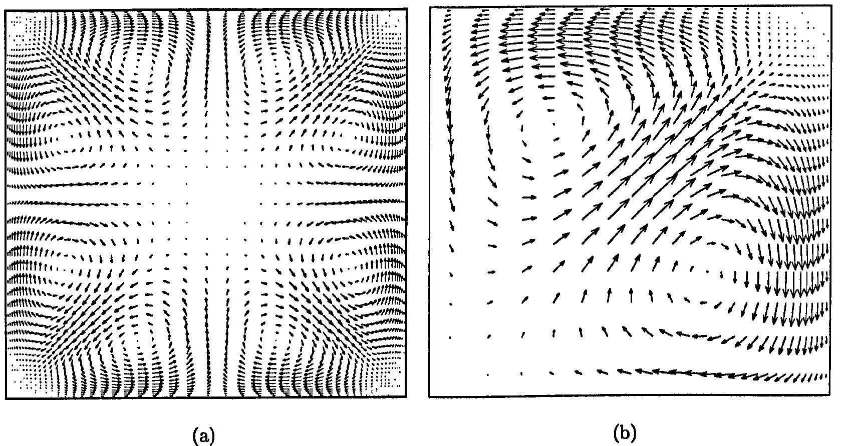
5.10 Secondary motions in a square duct using the EASM k-l
model: (a)
Full view and (b) zoom on the top right corner ... .... ... ... 86
5.11 Secondary motion in a square duct using the cubic eddy-viscosity model:
(a) Full view and (b) zoom on the top right corner . ... ... 87
5.12 Scalar trajectory in a 40 m long square duct .... ... 88
6.1 Overall view of the test room: (a) Top and (b) side view of the room
layout. 1: Filing cabinet, 2&3: desks, 4: DIN man, 5&6: Inlet ducts,
7: Door and 8: Outlet. Dimensions in mm
...
....
...
...
.
93
6.2 Ventilation layout and expected airflow pattern for the (a) displacement-
ventilation and (b) mixed-ventilation layout ...
....
...
94
6.3 Various dif£users. (a, b): "www. price-hvac. com", (c): "www. airtechproducts. com"
and (d): "www. poltech. com. au" .... .... ... ... .. 95
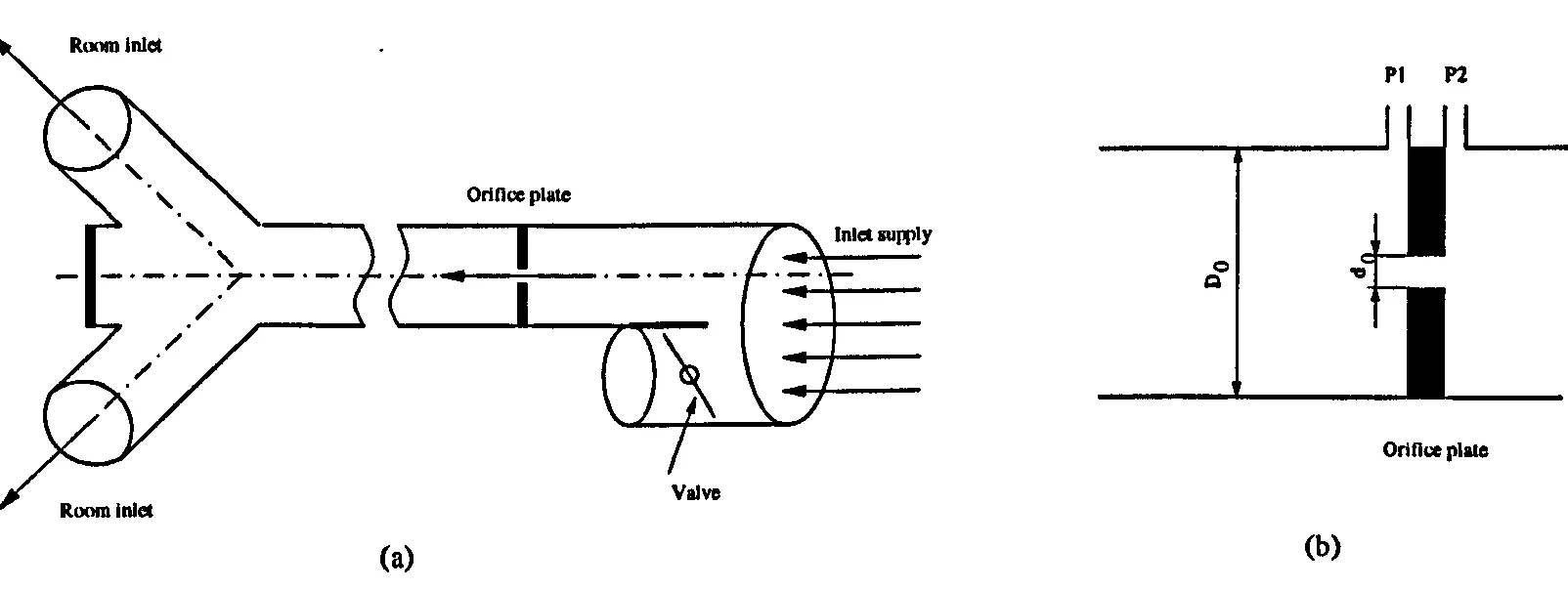
6.4 (a) Inlet duct system and (b) details of the orifice plate. ...
....
96
6.5 Schematic of the test facility
... 99
6.6 DIN man; (a) Standard cylindrical DIN man and (b) square cover...
.. 101
6.7 Dantec 54R10 transducer
.... ... .... ... .... ... 103
6.8 Location of the Dantec 54R10 transducers in the room. (a) Top view and
(b) side view of the room. Dimensions in mm
...
....
...
....
105
6.9 (a) Overview of the probes in the din man area with (b) projected view.
Dimensions in mm ... 106
6.10 Layout of the thermocouple in the room (marked by o); (a) Back wall,
(b) Front wall and door, (c) Left wall, (d) Right wall, (e) Floor and (f)
Ceiling. The hatched areas represent the room's furniture. Dimensions
in mm ... . .... ... .... . .... .... ... .... ... 108
6.11 Gas tracer analyser ... 109
6.12 Probe layout for the gas tracer analysis marked by o: (a) Overview and
(b) top view of the room. Dimensions in mm ... 111
7.1 Gas concentration in the room for Case 01 ... 114
7.2 Time-decay of gas concentration in the room for (a) Case 01, (b) Case 02
and (c) Case 03 ... ... .... ... .... .... ... ... 115
7.3 Time-decay of gas concentration in the room for (a) Case 04, (b) Case 05
and (c) Case 06 ...
....
...
....
....
...
. ....
116
7.4 Wall temperatures for Case 01: (a) back wall, (b) left wall, (c) right wall,
(d) floor, (e) ceiling and (f) door . .... ... ... .... 119
7.5 Thermal stratification in the room for Cases 01,02 and 03. ... 121
7.6 Thermal stratification in the room for Cases 04,05 and 06. ... 121
7.7 Inlet velocity measurements from the Dantec anemometers for Case 01.
. 124
8.1 Room geometry and position of vertical measurement axes (Dimensions in
mm). Distance from inlet along x: Al = 190 mm; A2 = 515mm; A3 =
965 mm; A4 = 1555 mm; A5 = 2355 mm ; A6 = 3155 mm; A7 = 3945 mm;
A8 = 4395 mm; A9 = 4720 mm ... 129
8.2 Comparison of predicted velocities with measurements (m/s)....
.... 131
8.3 Centerline velocity decay of the inlet jet: Comparison of measurements
with linear eddy-viscosity models . .... .... ... .... ... .... 132
8.4 Centerline velocity decay of the inlet jet: Comparison of measurements
with non-linear eddy-viscosity models . ... ...
...
....
134
8.5 Centerline velocity decay of the inlet jet: Comparison of measurements
with LES and LNS models . ...
...
...
..
134
8.6 Normal Reynolds stresses Txx/p along the jet centerline....
. ... 136
8.7 Normal Reynolds stresses Tyy/p along the jet centerline.. ... .... 136
8.8 Normal Reynolds stresses -rzz/p along the jet centerline.... ... .... 137
8.9 Centerline distribution
of a for the LNS model ... 138
8.10 Streaklines in the room. (a) Linear k-e, (b) cubic, (c) LES (Smagorinsky)
and (d) LNS models . ....
...
...
...
. ....
139
8.11 Velocity profile in the lower part of the room. (a) Profile A2, (b) profile
A4, (c) profile A6 and (d) profile A8
. ...
140
8.12 Contour plot of velocity at y+ -- 30 in the lower part of the room. (a)
Cubic model and (b) EASM k-e model
...
...
141
9.1 Shaw's room layout: 1: Partition; 2: Two desks; 3: Bookcase; 4: Filing
cabinet; 5: Inlet; 6&7: Outlets ... . ...
...
...
144
9.2 Time-decay of SF6 in the room. Measurements and predictions of eddy-
viscosity models in ak-1 framework ... ... ... 148
9.3 Velocity contour plots in the breathing zone (y = 1.6 m) for (a) k-1, (b)
cubic k-1, (c) k-e and (d) EASM k-e models ...
....
. ....
151
10.1 Room layout. (a) Three-dimensional view and (b) top view with location
of measurement points ... ... .... . .... .... . 155
10.2 Comparison of measured velocity profiles (a) M1, (b) M3, (c) M7 and (d)
M9 with predictions of the linear, EASM and cubic k-e models.
. ...
160
10.3 Comparison of measured velocity profiles (a) M1, (b) M3, (c) M7 and (d)
M9 with predictions of the linear, EASM and cubic k-l models. .... 161
10.4 Velocity contour plots in the room for (a) the linear and (b) EASM k-e
models ... ... .... ... .... ... ... . 162
10.5 Comparison of measured temperature profiles (a) M3, (b) M5, (c) M6
and (d) M8 with predictions of the linear, EASM and cubic k-e models. 164
10.6 Comparison of measured temperature profiles (a) M3, (b) M5, (c) M6
and (d) M8 with predictions of the linear, EASM and cubic k-I models. 166
11.1 Room layout: 1: Filing cabinet; 2: Large desk; 3: Desk; 4: DIN man; 5:
Outlet; 6: Door; 7: Light; 8: Mixed-ventilation inlet; 9: Displacement-
ventilation inlet ... 169
11.2 Averaged temperature stratification in the room for Case 01...
.
173
11.3 Averaged airflow temperature stratification in the room for Case 06.
..
174
11.4 Comparison of measured and predicted airflow velocities for Case 01.
..
175
11.5 Comparison of measured and predicted airflow velocities for Case 06. .. 176
11.6 Velocity contour plots in the DIN man's mid-plane for Case 01. (a) k-e
model and (b), instantaneous Smagorinsky LES
...
....
...
177
11.7 Velocity contour plots in the DIN man's mid-plane for Case 06. (a) linear
and (b) EASM k-e model . ...
...
...
...
....
177
11.8 Averaged concentration decay for Case 01
.... . ... ... 179
11.9 Averaged concentration decay for Case 06
.... ... .... ... .. 179
List of Tables
4.1 Alternate sweeping method for the TDMA solver
... ... 60
4.2 Number of iteration and computing time to reach convergence for test
case 2 and the simply ventilated room of He et al. (1999). . ... 67
5.1 Non-dimensional wall shear stress (T/(pUU) x 104). ....
... 72
5.2 Specifications of the backward-facing step flow
. ... ... 84
5.3 Specifications of the square duct used to obtain secondary motion..
... 85
6.1 Inlet velocity and temperature used during the experiments. ... . 98
6.2 Specifications of the Dantec 54R10 anemometer and requirements of the
ASHRAE and ISO 7726 (1985) standards
. ...
...
....
...
103
7.1 Location, mean temperature and velocity of the Dantec anemometers for
Case 01 (dimensions in mm) .... ... .... ... 123
7.2 Mean temperature and velocity of the Accusense thermistors for cases 01,
02 and 03 . ... .... ... .... .... ... ... 125
7.3 Mean temperature and velocity of the Accusense thermistors for cases 04,
05 and 06
. ...
...
....
....
. ....
...
....
...
126
7.4 Temperature of the Accusense thermistors taken as: T-T..,.. let.. .... . 126
8.1 Averaged prediction error at the jet centerline ... .... . ... 133
9.1 Room dimensions (m). Label 1-a to 1-d corresponds to the four sides of
the partition. Label 2-a ands 2-b are the two desks
...
145
9.2 Relative prediction error (%) of concentration decay for the models tested. 150
9.3 Ventilation efficiency index Ef at the time t= 20 mins..
...
152
10.1 Dimensions of the room configuration (dimensions in m).
...
157
10.2 Relative velocity error for each of the nine measured profiles..
...
163
10.3 Relative temperature error for each of the nine measured profiles.
....
167
11.1 Averaged wall temperatures for Case 01 and Case 06.
...
171
11.2 Coefficients of the polynomial fit for wall temperature of Case 01.
....
171
11.3 Averaged temperature error (%) of the models for Case 01 and 06..
...
175
11.4 Averaged velocity errors (%) ...
178
11.5 Relative averaged error (%) of the models compared with measurements. 180
11.6 Contaminant-removal
index
...
181
C. 1 Surface temperature in the, room for the displacement ventilation layout.
Dimensions in mm
...
222
C. 2 Surface temperature in the room for the mixed ventilation layout. Di-
mensions in mm ...
223
D. 1 Location, mean temperature and velocity of the Dantec anemometers for
Case 02 (dimensions in mm) ...
224
D. 2 Location, mean temperature and velocity of the Dantec anemometers for
Case 03 (dimensions in mm) ...
225
D. 3 Location, mean temperature and velocity of the Dantec anemometers for
Case 04 (dimensions in mm) ....
. ....
...
...
...
. ..
226
D. 4 Location, mean temperature and velocity of the Dantec anemometers for
Case 05 (dimensions in mm)
...
227
D. 5 Location, mean temperature and velocity of the Dantec anemometers for
Case 06 (dimensions in mm).
...
...
228
Nomenclature
a
Cross section area
A General coefficient solution of the discretised equations
Al to A12 Label for Accusense thermistors
A, Aµ
k-l
turbulence model constants
B
Wall roughness constant
B(;, j, k)
Spatial notation of grid points (Back)
Cl to C7
Non-linear eddy-viscosity model constants
C. Smagorinsky model constant
Cµ7 CEI, CE2
k-e model constants
Coo, Co, AE, Aµ k-l model constants
Cµ1, Cµ27 Cµ3 EASM coefficients
cw
Yap factor constant
d Length scale
D1 to D19 Label for Dantec anemometers
D, Discharge coefficient for orifice flowmeters
E Wall roughness constant
E(iJ, k)
Spatial notation of grid points (East)
F(ij, k) Spatial notation of grid points (Front)
ff, fl, f2
Damping functions
Gl to G5, GS, GR
Label of gas tracer sampling points
Gk
Buoyancy source term
H
Step height in backward-facing step flow
k
Turbulent kinetic energy
L Length scale
let lyc
Yap factor constants
im Mixing length
1s9,
Subgrid-scale length scale
lE
Dissipation length scale
1/.
& Eddy length scale
MW Molecular weight
N(1j, k)
Spatial notation of grid points (North)
p Average, or mean, pressure
P Instantaneous pressure
p' Fluctuating pressure
p* Guessed pressure for SIMPLE algorithm
pC Correction pressure for SIMPLE algorithm
Pk Production term
Pr Prandtl number
P(; j, k)
Spatial notation of grid points (Point)
R Ideal gas constant
[R]
Matrix of residual error
Re
Reynolds number
Ret, Rey Turbulent Reynolds numbers
S
Source term
Se
Extra source term for the E equation
Sid
Mean strain rate
Si*i Non-dimensional strain rate
Sij Resolved mean strain rate (LES)
S(ij,
k) Spatial notation of grid points (South)
T Temperature
T01 to T30 Label for thermocouples
t
Time
t; Turbulence time scale
U, V, W
Instantaneous velocities
u, v, w Averaged, or mean, velocities
u', V', W/
Fluctuating velocities
ic, IT, w
Time averaged velocities
ü, v, w Filtered velocities (for LES)
u*, v*, w*
Guessed velocities for SIMPLE method
u`, VC, wC Corrected velocities for SIMPLE method
u+ Non-dimensional velocity
V Volume flow rate
V* Velocity scale
W(i, i, k)
Spatial notation of grid points (West)
W=j
Mean vorticity rate
WZi Resolved vorticity rate (LES)
Wi*j
Non-dimensional vorticity rate
x, y, z
spatial coordinates
yC Yap correction factor
y+, y*
Non-dimensional wall distance
a RANS damping coefficient for LNS
al, a2, a3, g
EASM constants
Q Temporal discretisation parameter
Grid size or filter width for LES
b
Boundary-layer thickness
it Time step
b., bx, bx
Local grid spacing
b$i
Krondeker delta
rý, S
Invariance coefficients
e, E
Rate of dissipation of turbulent kinetic energy
Etiý Dissipation rate tensor
E8
Material emissivity
rk, I'E
Diffusion coefficients for k and c
ryl, 72,73 EASM constants
x
Von Karman constant
A Dynamic viscosity
At Turbulent viscosity
Atli µt2, µt3 Turbulent viscosity for EASM
/1898 Subgrid-scale turbulent viscosity
v Kinematic viscosity
S2
LNS parameters
IItj Pressure-strain correlation tensor
p
Fluid density
-PU SW
Turbulent scalar transport term
a
Stefan-Boltzman constant
vk, QE
Diffusion Prandtl numbers for k and e
Typ _ -piii Reynolds stress tensor
Ti7 Residual stress tensor (LES)
Tis 9s Subgrid-scale stress tensor (LES)
Typ Wall Shear stress
(D Instantaneous flow property
Mean flow property
Resolved flow property for LES
Fluctuating flow property
0893
Subgrid-scale flow property
0*
Guessed flow property used for SIMPLE method
c`
Corrected flow property for SIMPLE method
Subscripts
i, j, k Tensorial notation related to the spatial direction
1, m, n
Tensorial notation
g Multigrid level
nb Spatial notation of neigbouring grid points
x, y, z Spatial coordinates
Superscipts
sgs Subgrid-scale property
f
Finer multigrid level
Acknowlegmernts
I would like to thank my supervisor Paul Tucker for his kind help, guidance and
advice throughout the course of my PhD.
Special thanks to my dear friends Reza and Pascal who have always been there for help, support, and of course the occasional cheeky pint. As well as all the people I had the chance to meet and work with during my stay in Warwick, I would like to thank my friends Rai, Dr. Jason, Ross, Gianni and Helen, Rich, Karen, Yan and Mark who made the office a special place to work. I will never forget those friday afternoon coffees with Ross and Pascal nor will I forget the numerous CFD boys Ruby nights out.
Finally, I would like to thank my family and especially my parents whose uncondi- tional support carried me through the difficult, and the not so difficult, times of this PhD.
Declaration
I declare that the work presented in this thesis is my own work. This thesis or no
part of this thesis has been submitted for a degree at another University.
As part of the research, the following papers have been published:
. Jouvray A. and Tucker P. G., (2003), "On non-linear RANS, hybrid and LES
models applied to complex flows. ", Proceedings of the 4th International Symposium
on Turbulence, Heat and Mass Transfer, pp. 665-670, Ed. Hanjalic K., Nagano Y. and Tummers M., Begell House Inc., New-York, Swansea (UK).
" Tucker P. G., Liu Y., Chung Y-M. and Jouvray A., (2003), "Computation of
an unsteady complex geometry flow using novel non-linear turbulence models",
International journal for numerical methods in fluids, Vol. 43, No. 9, pp. 979-
1001.
" Liu Y., Tucker P. G., Jouvray A. and Carpenter P. W., (2003), "Computation of
a non-isothermal complex geometry flow using non-linear URANS and Zonal LES
modelling", Proceedings of the 3''d International Symposium on Turbulence and
Shear Flow Phenomena, Vol. 1, pp. 87-91, Ed. Kasagi N., Eaton J. K., Friedrich R., Humphrey J. A. C., Leschziner M. A. and Miyauchi T., Sendai, Japan, June, 2003.
" Holmes S. H., Jouvray A. and Tucker P. G., (2000), "An assessment of a range
of turbulence models when predicting room ventilation", Proc. Healthy Buildings
2000, Vol. 2, pp. 401-406, ISBN 952-5236-09-9.
Abstract
This thesis contributes to the numerical modelling of flows in ventilated rooms. A range
of advanced turbulence models (non-linear low Reynolds number Reynolds Averaged Navier-Stokes (RANS), Large Eddy Simulation (LES) and hybrid LES/RANS models)
are used to model the flow in four ventilated rooms. These describe the flow in a more
physically consistent manner than the commonly used linear RANS models.
The performances of Explicit Algebraic Stress Model (EASM) and, cubic eddy-
viscosity RANS model are first analysed on four benchmark flow configurations. They
show significant accuracy improvements when compared to their linear equivalents.
Flows in ventilated rooms are complex. Their numerical modelling required an accu-
rate definition of the various boundary conditions. This is often lacking in the literature
and hence, as part of this work, measurements in a controlled ventilated office (opti-
mised for Computational Fluid Dynamics (CFD) modelling) have been done. The mea-
surements comprise airflow velocities, temperatures, concentration decay and, a careful description of the room's boundary conditions under six ventilation settings. This room data is thus seen as ideal for validating of CFD codes when applied to room ventilation
problems.
The numerical investigations show that the predictions with zero- or, one-equation (k
- 1) RANS models (commonly used in room ventilation modelling) are less accurate
than those using two-equation k-e models. The study shows that the accuracy im-
provements of the EASM and cubic models are of lesser magnitude when applied to
room ventilation modelling than when applied to the benchmark flow configurations. The cubic model in particular, besides being more numerically unstable than the other
RANS models, does not always improve flow predictions when compared with its lin-
ear equivalent. The EASM, about 20 to 30% more computationally demanding than
its linear equivalent, improves solution accuracy for most flow considered in this work. LES predictions have highest level of agreement with measurements. LES is however
too computationally expensive to be used for practical engineering applications. The
novel hybrid RANS/LES model presented appears promising. It has similar accuracy
to LES at lower computational costs.
Chapter
1
Introduction
The research is concerned with airflows in ventilated spaces such as rooms and offices.
Ventilation
is used to control and maintain a specified air quality, air temperature,
moisture content, etc..., in a given space. To design an adequate ventilation system in a
building or a room, some knowledge of the airflow pattern is desired. Until the advent
of Computational
Fluid Dynamics (CFD) airflows in rooms were ascertained from an-
alytical methods, measurements or a-priori
knowledge from similar flow configurations.
With the growth of computer power, CFD methods have been applied to the modelling
of complex engineering flows. In the last
decade, CFD methods have been used as a de-
sign tool in the building industry to predict airflows. However, like in most engineering
flows, flows in ventilated areas are of a turbulent nature and cannot be easily modelled.
This work mostly contributes to the numerical modelling of turbulent flows in rooms.
Turbulence is a three-dimensional complex unsteady phenomenon. Turbulent flows
are characterised by the presence of large eddies which are created by the mean flow.
Another characteristic of turbulent flows pointed out by Leonard (1974), known as the
energy cascade, is that the energy of the
large eddies of the flow is successively dissipated
1 Introduction
2
`at 1ý
i ý1 ý 'äJ' 1ý ýt, _ºt ý iý __ r
WN-
Ott 4ý y rY ýI
cli
ýýý ýýý
yI }3
%) tyýý li
agrelAA ! "' lýN ýG' ýN .w.
Figure 1.1: Leonardo da Vinci's sketches on turbulence.
by smaller eddies. It is found that the smaller eddies of
the flow, near the Kolmogorov
scale, are universal whereas, the
larger eddies are highly dependent on the flow config-
uration itself (geometry, Reynolds number, etc...
). The modelling of the various eddy
scales is critical to ensure the correct energy
transfer within the fluid and hence predict
accurately flow fields.
From a historical perspective,
Leonardo da Vinci (1452-1519) is considered by many
as the first to study turbulence as
illustrated by his many drawings (see for example
Figure 1.1). Despite the efforts of many scientists such a
Newton (1643-1727) and
Bernoulli
(1700-1782) no mathematical models describing the turbulent motion of a
viscous fluid have been
found until the nineteenth century with the derivation of the
Navier (1785-1836) Stokes (1819-1903) equations. The Navier-Stokes (N-S) equations
[image:26.2112.416.1736.381.1316.2]1 Introduction
3
Reynolds (1842-1912) and Prandtl (1875-1953) have contributed to the development
of turbulence modelling techniques based on averaging methods. Another key contri-
bution of Reynolds (1842-1912) is the introduction of non-dimensional quantities, in
particular
the Reynolds number, to determine the state of fluid flows. The Reynolds
number is defined as Re = pud/p where p is the density of the fluid, ua characteristic
velocity, da characteristic length scale and p the viscosity of the fluid. The Reynolds
number expresses the ratio of inertial forces to viscous forces and is used to define the
laminar state (at low Reynolds number) or turbulent state (at high Reynolds number)
of a fluid.
The transition from laminar to turbulent flow, which typically occurs at
Re, = 1.3 x 10⁵ - 1.3 x 10⁶ for a flat plate boundary layer, is complex and governed
by the growth in space and time of Tollmien-Schlichting instabilities. Further details on
transition processes is extensively covered in the literature (i. e. Schlichting and Gersten
(2000), Tritton (1988)).
The contribution of the many researchers over centuries has given rise to a math-
ematical expression of fluid motion as the conservation of three physical quantities:
Momentum,
mass and energy. These equations are the governing equations of fluid
flows and are expressed here in their incompressible form as:
avi
+
avi u;
1 ap za (av= av;
ät
ax; =-pTx
+pax;
lax; +ax; l
(i. iý
au;
axe
(1.2)
a(AT)
9(pTUj)
(9
it
_
OT
at
+
axi
öxj
P,. axe)
(1.3)
The momentum equation (Equation 1.1) is commonly referred as the N-S equation and
is the expression of Newton's second law. Equation 1.2 is commonly referred as the
1 Introduction 4
the energy equation and embodies (via the Reynolds transport theorem) the first law of
thermodynamics.
The computation of turbulent flows using the governing equations can be achieved
using either of the three following methods: Direct Numerical Simulation (DNS), LES
or the BANS method.
DNS is the resolution (through the use of extremely fine grids and time steps) of
the full N-S equations for all time scales and spatial scales of a given flow. As a result,
DNS provides highly accurate results but suffers greatly from being computationally
expensive. DNS requires a grid resolution of the order of the Kolmogorov scales and
needs a grid resolution of the order of = 1013 for airflows in rooms (Zhang and Chen
(2000)). Due to the limitations of computing power and because the computational
cost of DNS increase as Re 3 (Pope(2000)), DNS is still limited to the resolution of low
Reynolds numbers flows and is thus not considered in this work.
To reduce computational cost and resolve more complex flows at higher Reynolds
numbers, methods to approximate the consequences of turbulence are used. LES and
RANS methods are currently the two most popular methods for computing practical
turbulent flows. The numerical work presented here focuses on RANS, LES and hybrid
RANS/LES approaches. A brief overview of these methods is given below and further
discussed in Chapter 3.
In LES, a separation of scales is assumed for the flow eddies. The larger are com-
1 Introduction
5
(i. e. Smagorinsky (1963), Deardorff (1974)) was aimed towards meteorological applica-
tions and atmospheric boundary layers. An extensive overview of LES and its applica-
tions to atmospheric modelling can be found in Galperin and Orzag (1993). With recent
increases in computing power, LES has become increasingly popular for the modelling
of flows at low to medium Reynolds numbers. LES for ventilated rooms is presented as
part of this work.
The third and most popular method for computing turbulent flows is based on a form
of time averaging of the governing equations. The averaging of the governing equations
introduced by Reynolds (1895) (further described in Section 3.1) yields the RANS equa-
tions. These can be solved for most flow configurations and Reynolds numbers. The
averaging of the governing equations, however, removes some of the key information on
the time dependent fluctuations of the flow itself. Therefore, predictive accuracy can
be relatively low. However, RANS solutions are relatively inexpensive. A wide range
of BANS models is found in the literature
(see Wilcox (1995)). Linear eddy-viscosity
models such, as the k-E
model (see Chapter 3), have been widely validated but have
limitated prediction accuracy. Their application to the modelling of ventilated rooms
is reviewed in Chapter 2. The numerical prediction of flows in rooms using RANS here
focuses on models that include a more consistent description of turbulent flow physics
(i. e. non-linear eddy viscosity models and those derived from Reynolds stress models).
Part of this work aims to assess the range of applicability and accuracy of these advanced
RANS models. To do so, they are first validated using known data of four benchmark
1 Introduction
6
To enhance flow predictions and keep computational cost to a minimum, zonal and
hybrid RANS/LES
methods are tested. In zonal models, computational
expense is re-
duced by solving the computationally demanding near-wall areas using RANS. This
region is demanding using LES since it contains fine streak-like structures needing an
especially fine grid to resolve (see Chapter 3). The remainder, or core, of the flow is
solved using LES. In hybrid models the transition between RANS and LES can occur
at any point of the domain. Hybrid models are discussed in Chapter 3.
To fully assess the performances of numerical models, comparison with experimental
data in a realistic ventilated spaces is required. It is often found in the literature that
measurements in ventilated rooms are not well suited for CFD modelling. These often
have missing boundary condition definition and hence cannot be used for the evaluation
of numerical models. Thus, as part of this work, measurements in a ventilated office
idealised for CFD modelling are made. For these, the boundary conditions are carefully
defined.
Layout
of the thesis
A general introduction to room ventilation processes and a review of CFD modelling
applied to room ventilation is presented in
Chapter 2. Chapter 3 presents the RANS,
LES, zonal and hybrid RANS/LES models (equations and physical underlying prin-
ciples) used. An overview of the numerical methods used is given in Chapter 4. In
Chapter 5, the advanced RANS models as implemented in the code are assessed in
terms of accuracy and range of applicability for four benchmark problems. Chapter 6
1 Introduction
7
office. Finally, Chapter 8 to 11 present the numerical investigation of four ventilated
rooms. In Chapter 8, a wide range of turbulence models is applied to a simple empty
jet-ventilated
room. The performances of RANS models for the time-decay predictions
Chapter
2
Literature
review
2.1
Introduction
to room-ventilation
processes
Until recently (early 1970's), the vast majority of offices and buildings in the U. K. were
naturally ventilated (Awbi (1996)). The increased interest in improving ventilation sys-
tems in buildings, rooms and offices, in the last decades, has been driven by three key
elements, namely the availability of relatively inexpensive energy sources, the increased
need for improving comfort and well being in working places and the increased aware-
ness of the impact of air quality on the health of people. These factors remain key in
the definition of modern ventilation systems which aim to provide occupants a suitable
air quantity, air quality and thermal comfort at low energy costs.
From a practical point of view, the ventilation of rooms can be grouped under two
main categories: Natural ventilation and mechanical (or forced) ventilation.
It is often
found that in real buildings, a combination of the two techniques is used.
The growing awareness of environmental issues is leading to tremendous changes in
2.1 Introduction to room-ventilation processes 9
[image:33.1936.346.1568.363.1296.2](a)
Figure 2.1: Naturally ventilated buildings: Computational
model of the Hall of Still
Thought in Taiwan. (http: //www. architectureweek. com/).
building architecture in modern cities. Naturally ventilated buildings are becoming a
popular choice. They have the main advantage of being highly energy efficient and so,
environmentally friendly. Natural ventilation in buildings is caused by external winds
or buoyancy forces between the inside and the outside of the building (Croome and Roberts (1981)). Naturally ventilated buildings or rooms are, however, not as versatile
nor as stable as mechanically ventilated buildings. In order to be efficient, their de-
sign, as illustrated by Figure 2.1, is often found to be of a complex nature. Mechanical
ventilation systems provide a better controlled indoor climate than natural ventilation
systems. Natural ventilation is often used for large-scale ventilation (i. e. a building as
a whole) and mechanical ventilation systems are often used for the specific needs of a
2.1 Introduction to room-ventilation processes 10
Mechanical ventilation systems are mainly composed of a fan, a temperature regu-
lation unit, an air-filtering device, a fresh air supply and, of inlet and outlet diffusers
placed in the room. This study is only concerned with the ventilation processes occur-
ring inside rooms or offices and further details on the various components constituting
a mechanical ventilation unit can be found in McQuiston and Parker (1994) and Jones
(1997). The mechanical ventilation of rooms is found under many forms that mainly
differ from each other by the layout and shape of the various inlets and outlets in the
room. The influence of the diffuser on the airflow pattern in a room is illustrated by Hu,
Barber and Chuah (1999) who studied numerically, using the k-e turbulence model
with a condensation and thermal comfort model, the indoor environment provided by
three diffusers. The airflow pattern in the room as well as the thermal comfort analysis
is found to be highly dependent on the diffuser. Further discussion on inlet diffusers is
found in Chapter 6.
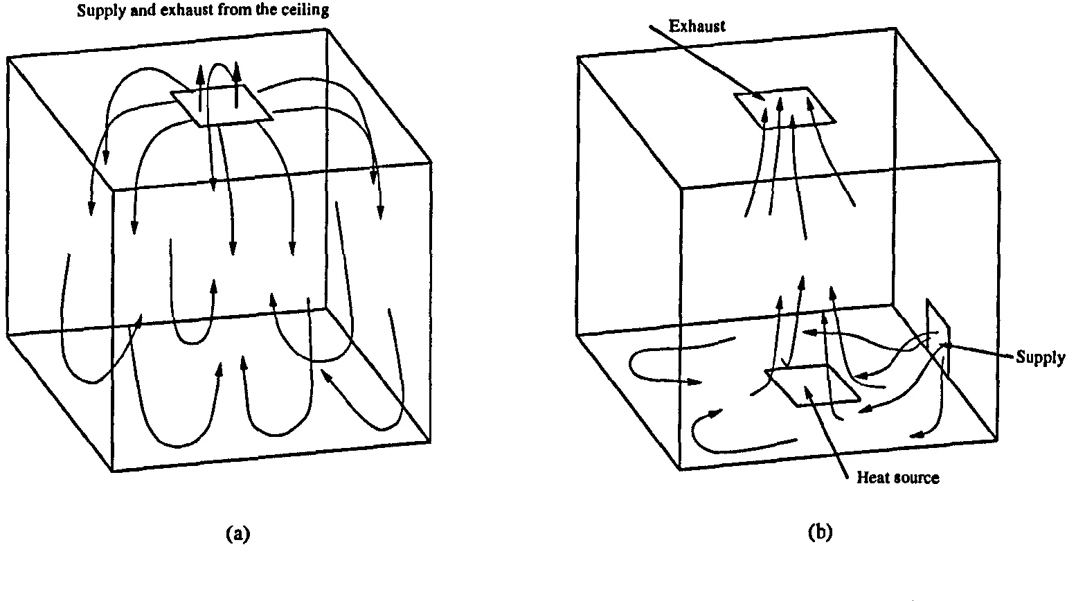
The two dominant ventilation layouts illustrated by Figure 2.2 are displacement- and
mixed-ventilation. A mixed-ventilation layout (Figure 2.2 (a)) consists in the supply and
exhaust of air in the ceiling area of the room. In mixed-ventilation, the air is supplied at
higher velocity than in displacement-ventilation and creates a uniform (mixed) indoor
environment. The presence of an extraction fan on the mixed-ventilation device ensures
an adequate air renewal in the room. In a typical displacement-ventilation layout, as
illustrated by Figure 2.2 (b), cold air is supplied at low level and returned in the ceiling
area. The airflow pattern of displacement ventilated areas is governed by convection
phenomena. When the cool supplied air encounters heat sources, (such as a working
2.1 Introduction to room-ventilation processes 11
(a) (b)
Figure 2.2: Typical ventilation layouts: (a) Mixed-ventilation and (b) displacement-
ventilation layout.
room is thus driven by the rise of air from the lower part to the higher part of the room.
Mundt's (2000) investigation in a displacement ventilated room shows that particles
introduced at a low level, and therefore subject to convection, do not increase drastically
the risk of polluting the breathing zone of a standing or walking individual. However,
the motion of an individual is found to increase the concentration of particles in the
breathing zone and outside the convective area. It is also found that the decay rate of
larger particles (> 10µm ) is mostly independent of the convective flow.
Xing, Hatton and Awbi (2001) compare the overall air quality in a displacement
ventilated room, equipped with various heat load and a thermal manikin, with the air
quality in the breathing zone. Both numerical predictions (standard k-e model) and
[image:35.1936.174.1741.361.1229.2]2.1.1 Air quality
12
measurements are used. The investigation shows that the air quality in the breathing
zone is better than the overall air quality in the room (up to 50% better for a seated
manikin and up to 20% better for a standing manikin) and highlights the advantages of
the displacement-ventilation layout.
The next sections place greater emphasis on CFD work in relation to air quality
issues, thermal comfort and ventilation effectiveness in rooms. Recent developments in
CFD methods allows better flow predictions but, the trade-off between prediction ac-
curacy and computational expenses remains crucial in the industrial world. Thus, most
of the CFD work undertaken for room ventilation, and presented here, is carried out
using linear eddy viscosity BANS approach and in particular the standard k-e turbu-
lence model (see Chapter 3). Only recently the use of more advanced approaches for
the modelling of turbulence, such as variants of the standard models or LES, have been
applied to simply ventilated room or offices. These novel CFD techniques as applied to
room ventilation are reviewed in Section 2.2.
2.1.1
Air quality
Air quality issues in ventilated areas has become a topic of great interest in the last
decades with studies revealing the association between indoor air quality and numerous
health complaints. In particular the Sick Building Syndrome (SBS) which can be traced
back to 1970 (Hart (1970), LaVerne (1970)) has been extensively covered in the recent
years (i. e. Sundell (1996), Hedge (1992), Molhave (1989)). The SBS as defined by the
World Health Organization (WHO (1983)) includes a range of symptoms such as skin,
2.1.1 Air quality
13
lated with ventilation rate, air quality and airflow patterns in a room (Sundell (1994)).
Besides the SBS, air quality issues in rooms and offices are often related to the diffusion,
containment and extraction of pollutant sources. A typical list of pollutant sources in
rooms such as CO2i smoke, radon, etc... is given by Hodgson (2000).
The control of the diffusion of contaminant sources (i. e. Environmental Tobacco
Smoke (ETS), airborne viruses, etc... ) is one example where ventilation is needed. The
extraction and control of ETS in public places has become a greater problem in the
last decades as illustrated by the new amendments to the Norwegian Smoking Law of
1988. The latter stipulates that at least one-half of the tables in a restaurant are to be
kept free of smoke. Some of the basic ventilation rules and strategies to adopt where
both smoking and non-smoking people share a common space is reviewed by Krühne
and Fitzner (2000). One of the problem induced by investigating the diffusion of ETS
products is that it is constituted by a range of particles sizes which, as showed by Mundt
(2000), have a different distribution in a ventilated area.
Mundt's (2000) work on particle distribution is further supported by Timmer and
Zeller's (2000) investigation. The numerical simulation of Timmer and Zeller (2000)
compares predicted deposition of particles in the vicinity of the outlet of a ceiling inlet,
floor outlet ventilation system with the experimental data of Rauer (1996). Rechnagel
et al. (1999) estimate that one million solid particles are contained in 1 m3 of air in
an average European city. 98% of these particles have a diameter of less than 1 pm
and represents only 3% of the total mass load. The numerical modelling of Timmer
and Zeller (2000), using the commercial code FLUENT/4.48TM with a particle load of
2.1.1 Air quality 14
particles sizes in the range 0.1 to 40 pm. The increase of particle load from 800 to 1400
g/m3 increases particle deposition from 1% to 2.4%. A rise in the inlet velocity from
2.4 to 4.7 m/s increases the amount of deposited particles from 0.1% to 2.5%. Finally,
the increase of the outlet turbulence intensity from 2 to 80 also increases the amount of
particles reaching the ceiling from 0.5% to 3.3%. These results are found to be in good
agreement with the experimental data of Rauer (1996) and emphasise the importance
of the turbulence level, velocity and particle size on the deposition of particles in a ven-
tilated room.
Thus, to analyse accurately the diffusion of complex pollutants such as ETS in venti-
lated spaces, experimental data on the size and quantity of these particles are required.
Experimental data such as those of Cumo et al. 's (2000) which relate the nature and
variation of the concentration of ETS in the house of parliament in Rome can be used
to validate numerical methods. Other studies on particles distributions in rooms can be
found in Nazaroff et al. (1990), Lu (1995) and Lu and Howarth (1999) who investigate
numerically, using the k-c model, the particle distribution in a multizone ventilated
room.
One of the most efficient way to contain the diffusion of smoke in a given space is
to install obstacles or partitions. Air curtains, as often seen in commercial buildings
and warehouse, are designed to maintain thermal comfort at low energy expenses. Air
curtains can also be used as an obstacle or partition that separates smoking and non-
smoking areas. Rydock et al. 's (2000) investigation is based on the design and evaluation
of an air curtain that aims to isolate smoking and non-smoking areas in a restaurant.
2.1.1 Air quality 15
smoking area but, a completely smoke-free area could not be achieved.
Changes in legislation in recent years also affect ventilation rates required in public
places. Among the many changes, ventilation rates in classrooms have been affected as
illustrated by the amendment of building regulations in the U. K. (2001) which imposes
a minimum of 3 litres of fresh air per second per occupant.
The recent interest- in classroom ventilation can be illustrated by the work of Zeng
et al. (2000) who investigate experimentally and numerically the flow behaviour inside
a typical Canadian portable classroom equipped with a single high-mount supply and a
single low-mount exhaust ventilation device. The experimental data (flow visualisation
and SF6 measurements) are used for the implementation of the boundary conditions
of the three-dimensional CFD simulation (standard k-e model). The unsteady CFD
model is used to predict the mean age of air and CO2 concentration in the room. The
latter, since stagnation zones with high CO2 concentrations are observed at the front of
the classroom, underlines the need for improvement of the ventilation unit.
Karimipanah et al. (2000) study the efficiency of four ventilation strategies (displacement-
ventilation, mixed-ventilation, impinging jet and textile diffuser) in a mock-up of a full-
size classroom under the extreme external temperature conditions found in Sweden.
Both experimental analysis and CFD modelling (k -e model of the VORTEX code) are
made. CFD and experimental data are found to agree well. The minor discrepancies
observed are partly explained by the strong buoyancy effects induced by the ventilation
device and, by the lack of accuracy of the CFD model especially in the near-wall areas. It
2.1.2 Thermal comfort 16
2.1.2
Thermal
comfort
Ventilation also aims to increase thermal comfort in rooms and offices in order to in-
crease the level of productivity of its occupants (Awbi (1991)). Since the sensation of
comfort depends on the individual thermal comfort is a difficult topic to address scien-
tifically. To understand and study thermal comfort, a series of parameters or indices
have been introduced over the years to define the level of satisfaction of the room's
occupants (Fanger et al. (1988)). The Predicted Percentage of Dissatisfied (PPD) and
Predicted Mean Vote (PMV) are among the standard indices used. Thermal comfort
in a room depends on a multitude of parameters such as ventilation strategy, clothing,
body activity, etc... . The ISO 7730 (1994) and ASHRAE (1993) standards offer some
guidelines on indoor temperature settings based on ideal experimental conditions. These
guidelines are often found to be misleading when considering real rooms (Awbi (1998)).
Thermal problems in ventilated rooms can mostly be assimilated as thermal plumes
rising from sources such as lighting, electrical equipment, etc... . Using the water tank
analogy, Hunt et al. (2000) investigate the variations in the mixing process of a non-zero
momentum buoyancy point source. This problem, commonly referred as the filling box,
is carefully described by Baines and Turner (1968) and includes most of the physical
behaviour of thermal problems encountered in rooms. Hunt et al. 's (2000) experimental
analysis reveals that buoyancy effect alone leads to a stable flow stratification in the
room. The combination of buoyancy and momentum sources (or jet) leads to a more
traditional jet flow, to unsteadiness and, drastically affect the overall thermal behaviour
2.1.2 Thermal comfort 17
Park and Holland (2000) perform a two-dimensional numerical simulation (k -E
model) of a heat source in a displacement ventilated room. The investigation aims to
determine the influence of the position of the heat source on the performances of the
ventilation system. As expected the CFD results show that, since both buoyancy forces
and momentum effects are present (c. f. Hunt et al. (2000)), the thermal plume gener-
ated by the heat source is affected by the displacement-ventilation inlet. It is found that
the height of thermal stratification reduces as the heat source rises. The temperature
gradient observed near the ceiling is found to increase as the heat sources rises. This
also increase the cooling load required to maintain the room's temperature.
Thermal comfort in displacement ventilated areas is difficult to achieve. This is
illustrated by Melikov and Nielsen (1989) who analysed thermal comfort in 18 displace-
ment ventilated spaces. They found that up to 15% of occupants are dissatisfied due
to draught problems. Also, about 40% of the locations considered have a thermal gra-
dient > 3K between the head and feet of the occupants. To enhance predictions of
thermal stratification and thermal comfort in displacement ventilated rooms, Yuan et
al. (1999) created a large database of air temperature and contaminant distribution in
various rooms. This is further discussed in Chapter 10. Using this database, Yuan, Chen
and Glicksman (1999) developed simple models that aim to determine the temperature
stratification in typical displacement ventilated offices.