University of Warwick institutional repository: http://go.warwick.ac.uk/wrap
This paper is made available online in accordance with
publisher policies. Please scroll down to view the document
itself. Please refer to the repository record for this item and our
policy information available from the repository home page for
further information.
To see the final version of this paper please visit the publisher’s website.
Access to the published version may require a subscription.
Author(s):
M. Mathioudakis, D. S. Bloomfield, D. B. Jess, V. S. Dhillon,
and T. R.Marsh
Article Title: The periodic variations of a white-light
flare observed with ULTRACAM
Year of publication: 2006
Link to published article:
http://dx.doi.org/10.1051/0004-6361:20054752
DOI: 10.1051/0004-6361:20054752 c
ESO 2006
Astrophysics
&
The periodic variations of a white-light
flare observed with ULTRACAM
M. Mathioudakis
1, D. S. Bloomfield
1, D. B. Jess
1, V. S. Dhillon
2, and T. R. Marsh
31 Department of Physics and Astronomy, Queen’s University Belfast, Belfast, BT7 1NN, Northern Ireland, UK e-mail:[email protected]
2 Department of Physics and Astronomy, University of Sheffield, Sheffield, S3 7RH, UK 3 Department of Physics, University of Warwick, Coventry, CV4 7AL, UK
Received 22 December 2005/Accepted 19 April 2006
ABSTRACT
High time resolution observations of a white-light flare on the active star EQ PegB show evidence of intensity variations with a period of≈10 s. The period drifts to longer values during the decay phase of the flare. If the oscillation is interpreted as an impulsively-excited, standing-acoustic wave in a flare loop, the period implies a loop length of≈3.4 Mm and≈6.8 Mm for the case of the fundamental mode and the second harmonic, respectively. However, the small loop lengths imply a very high modulation depth making the acoustic interpretation unlikely. A more realistic interpretation may be that of a fast-MHD wave, with the modulation of the emission being due to the magnetic field. Alternatively, the variations could be due to a series of reconnection events. The periodic signature may then arise as a result of the lateral separation of individual flare loops or current sheets with oscillatory dynamics (i.e., periodic reconnection).
Key words.waves – stars: activity – stars: atmospheres – stars: flare – stars: individual: EQ Pegasi
1. Introduction
The detection of oscillations in coronal loops has provided clear evidence for waves in the upper solar atmosphere (Nakariakov & Verwichte 2005). These observations provide new insights into the processes of atmospheric heating. They have also raised the prospect of using oscillations as a diagnostic to infer the proper-ties of the upper solar atmosphere and allowed the development of coronal seismology (Roberts 2000). For example, Nakariakov & Ofman (2001) developed a method for determining an abso-lute value for the magnetic field strength of coronal loops that oscillate as a result of standing kink-mode waves. The crucial theory of MHD oscillations in solar atmospheric structures has been presented by Roberts et al. (1984), where both standing and propagating wave modes are considered. Coronal structures, such as the loops within an active region, can act as wave guides supporting quasi-periodic variations (Roberts et al. 1983).
There is increasing evidence to suggest that oscillations in the solar atmosphere can be triggered by flares and other nearby impulsive events. Kane et al. (1983) observed 8 s pulsations of large amplitude during the hard X-ray (HXR) and microwave bursts of a solar flare, while McKenzie & Mullan (1997) have re-ported periods of 10−60 s in the active, non-flaring solar corona. Schrijver et al. (2002) have shown that oscillation events ob-served by theTransition Region and Coronal Explorer(TRACE) are often triggered by flares and filament eruptions, occurring in closed coronal loops with no clear dependence of the oscil-lation amplitude on the magnitude of the flare. Lower in the at-mosphere, McAteer et al. (2005) have shown that a flare induced an oscillatory signal along an Hαribbon.
The solar analogy is often used to interpret the wide range of phenomena observed in active stars. Quasi-periodic fluctuations (≈30 s) of varying amplitude were reported in the quiescent state
of active flare stars and were considered to be a signature of mi-crovariability (Andrews 1989). A similar study by Mullan et al. (1992) reported periodicities of a few minutes which were inter-preted as transient oscillations in coronal loops. There are also some reports of periodic intensity variations during stellar flares. Short duration variations (10−20 s) were reported after the onset of a strong flare on the Hyades star II Tau (Rodonó 1976), while Mathioudakis et al. (2003) reported a large amplitude periodicity (220 s) during the peak of a flare on the RS CVn binary II Peg. The first stellar flare oscillation in X-rays was recently reported by Mitra-Kraev et al. (2005).
Quasi-periodic oscillations during flares can be generated by both the second harmonic of the acoustic mode (Nakariakov et al. 2004; Tsiklauri et al. 2004) and the fundamental mode (Taroyan et al. 2005). The numerical modeling shows that the loop density exhibits perturbations with a maximum near the loop apex, with the oscillation period dependent on the ratio of the loop length to the sound speed (Roberts et al. 1984). This approach is particularly useful when applied to stellar flares as it provides a method for determining the spatial dimensions of stellar coronal loops.
EQ Peg (Gl 896AB) is a visual binary system with a separa-tion of 5. Both components are M-type flare stars with visual magnitudes of 10.3 and 12.4, respectively. Flare activity on the system has been observed over a large part of the electromag-netic spectrum from X-rays to radio wavelengths. In white light, the flare frequency of the binary is∼0.8 flares h−1for flares with energy in excess of 1030erg (Lacy et al. 1976).
Small-amplitude stellar variations are often met with some skepticism as they may be due to sky fluctuations. To bypass this difficulty multi-site observations may be used (Zhilyaev et al. 2000). Here we use high-cadence, multi-wavelength photometry to study periodic intensity variations during a flare on EQ PegB.
324 M. Mathioudakis et al.: Flare oscillations
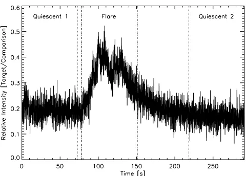
Fig. 1.Theu-band lightcurve of the analyzed flare on EQ PegB. Time is given in seconds since 21:32:53 UT on November 4th 2003.
Synchronous observations of a comparison star were obtained in order to remove any atmospheric variations. Section 2 details the instrumentation and observations, with the form of time series analysis presented in Sect. 3. The results are discussed in Sect. 4, while our conclusions are drawn in Sect. 5.
2. Observations and data reduction
The observations presented here were obtained with the triple-beam CCD instrument
ultracam
(Dhillon & Marsh 2001). The instrument uses two dichroic beam-splitters to separate the light into three wavelengths which pass through differing Sloan (sdss
) filters. The detector system comprises of three back-illuminated Marconi 1024×1024 frame-transfer CCDs, allow-ing the collection of data in the imagallow-ing area while data in the masked area is read out. Each chip is triggered by the same GPS synchronized system clock.We used
ultracam
on November 4th 2003 with the 4.2 m William Herschel Telescope on La Palma, resulting in a spa-tial sampling of 0.3 pixel−1. The large imaging area of the CCDs allows simultaneous observations of the target and a suf-ficiently bright comparison star. Smaller windows of 21×21 were used around these objects to minimize the dead time be-tween exposures. The observations were made in theu,g, and r Sloan passbands with an exposure time of ∼0.073 s. The data were reduced with theultracam
pipeline reduction soft-ware. The pipeline uses aperture photometry to produce separate lightcurves for each selected object within the field of view (i.e., both the target and the comparison).3. Time series analysis
The u-band lightcurve of the flare on EQ PegB is shown in Fig. 1, where the duration of the flare is≈160 s. The impul-sive phase of the event is followed by intensity variations which were analyzed by both a Fast Fourier Transform and a wavelet transform. Although wavelet analysis is similar to a windowed Fourier analysis, the latter may be considered as an inefficient method for the study of quasi-periodic oscillations. This arises not only from Fourier analysis comparing different numbers of oscillatory cycles for differing analysis frequencies, but the win-dowing process imposes a shorter time interval on the time series within which the analysis is carried out. Hence, the frequency
resolution of the Fourier analysis is degraded since∆ν = 1/T, whereT is the analysis duration.
With wavelet analysis the search for periodic signatures is carried out by a time-localized function which is continuous in both frequency and time (Torrence & Compo 1998), mak-ing it well suited for the identification of transient oscillations. Wavelets have become the preferred analysis technique in recent years because wave phenomena in solar and stellar atmospheres have finite durations. An extensive discussion on the effects that various wavelet parameters have upon their results is given in De Moortel et al. (2004).
The wavelet used in this study is the Morlet function, which is defined as the product of a complex exponential (i.e., sine) wave with a Gaussian envelope,
ψt(s)=π−1/4exp (iωt) exp
−t2 2s2
, (1)
wheretis the time parameter,sis the wavelet scale (related to the Fourier period byP =1.03 s for the Morlet function),ωis the oscillation frequency parameter, andπ−1/4 is a normaliza-tion term (Torrence & Compo 1998). By varying the scale of the wavelet function (i.e., both the Gaussian width and the oscil-lation period) such that the sinusoidal portion matches a given oscillation frequency, the wavelet is convolved with the time se-ries to determine the contribution of that frequency to the time series. At each wavelet scale, the timing information is achieved by scanning the wavelet function through the time series.
The portions of the u,g, andr time series occurring be-tween the vertical dot-dashed lines in Fig. 1 were filtered using wavelet reconstruction to remove the long-period power associ-ated with the general flare profile. This technique rebuilds the time series,xt, from the wavelet transform,Wt(s), using only
in-formation from the desired scale values,sj,
xt=
δjδt1/2 Cδψ0(0)
J
j=0
{Wt(sj)}
s1j/2 , (2)
where δj defines the degree of frequency sampling (taken as 1/32 here),δt is the cadence (0.073 s), and bothCδ andψ0(0) are constants (0.776 and π−1/4 for the Morlet wavelet, respec-tively). The time series presented here were reconstructed over all scale values corresponding to periods less than 17 s, a point discussed in more detail later. The wavelet power transform of our filteredu-band time series is shown in Fig. 2 where regions of lighter shading indicate greater oscillatory power. The cross-hatched area is the cone of influence (COI) and defines the region of the power spectrum where edge effects may become impor-tant due to the finite duration of the time series – the extent of the COI at each period is thee-folding or decorrelation time of the wavelet function.
The reliability of any oscillatory power seen in our data is tested against a number of criteria:
1. Power is tested against spurious detections which could be due to Poisson noise. The contours in Fig. 2b outline the power at which detections are 99% confident using a two de-gree of freedomχ2distribution.
Fig. 2. a)The filteredu-band time series.b)The Morlet wavelet power transform of the time series ina)as a function of both time (abscissa) and oscillation period (ordinate). Contours define the power above which detections are 99% confident using a two degree of freedom χ2distribution.c)The global (i.e., averaged) wavelet power (full line) and Fast Fourier power (crosses) as a function of period. The 99% con-fidence levels are over-plotted for the global wavelet and Fourier curves as dot-dashed and dotted lines, respectively.
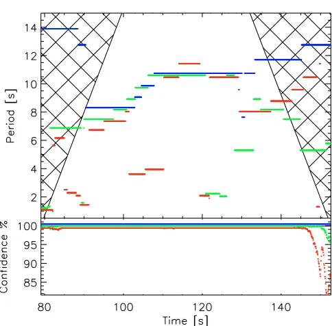
times that the random series produce equal or greater power than the actual data – high values indicating no periodic sig-nals in the data while low values suggest the detected peak power periods are real. Confidence levels are calculated from (1−p)×100 and are shown for each of our time series in the lower panel of Fig. 3.
3. As mentioned previously, the extent of the COI is the decor-relation time of the wavelet function. For the Morlet wavelet this is √2P, wherePis the oscillatory period. The choice of cutoffperiod for the filtering (17 s) was based on this value, as longer periods (i.e., those above the dashed line in Fig. 2b) can not exist for a decorrelation duration outside the COI. To minimize the chance of detecting noise spikes, we require real detections to have power above the 99% confidence level for at least three oscillatory cycles (i.e., two decorrelation durations).
4. Results and discussion
Our analysis shows a reliable oscillation with a period of≈10 s during the flare on EQ PegB. The oscillation starts just before flare maximum (t≈100 s) and continues into the decay phase. We conclude that it is due to white-light continuum variations rather than the Balmer and Ca
ii
H&K lines which can provide a significant contribution to theu-band flux during a flare, be-cause it is seen in all three bands (u,g, andr). The following interpretations may be considered.4.1. An impulsively-generated acoustic wave
[image:4.595.301.543.68.306.2]The generation of standing, slow-mode waves in active, coro-nal loops which are anchored in the photosphere was first pro-posed by Roberts et al. (1984). Assuming both a strong longi-tudinal component (in order to yield density and hence intensity variations) and that the magnetic field dominates sufficiently to
Fig. 3.Upper: oscillation period exhibiting the peak wavelet power at each point in time.Lower: confidence levels achieved by peak wavelet power through randomization testing. In both panels the results from theu(blue),g(green), andr(red) bands are plotted separately.
approximate the longitudinal tube speed with the acoustic speed, the period of a standing, slow-mode oscillation is given by,
P(s)≈ L(Mm)
7.6×10⁻²N√T(MK), (3)
where T is the average temperature along the loop, L is the length of the loop, andNis the mode of oscillation (i.e., 1 yields the fundamental mode, 2 the second harmonic). In Fig. 3 we show the oscillatory periods exhibiting the maximum power at each point in time. In all three
ultracam
bands, the pe-riod shifts to longer values during the decay phase of the flare. This behaviour can be explained by the standing, acoustic-wave model as a result of a temperature decrease and/or increase in loop length after the flare peak. Substituting the detected oscil-lation period (10 s) and a temperature of 20 MK into Eq. (3) we obtain a loop length of≈3.4 Mm (0.015R) for the fundamental mode and≈6.8 Mm (0.030R) for the second harmonic.In a recent numerical model, Nakariakov et al. (2004) have shown that the standing second harmonic of an acoustic wave can be excited in a flaring loop. The excitation of these oscilla-tions is almost independent of the location of the heat deposi-tion in the loop (Tsiklauri et al. 2004) and appears as a natural response of the loop to an impulsive energy deposition. Taroyan et al. (2005) have also examined the excitation of acoustic waves as a result of an impulsive energy deposition at the chromo-spheric footpoint of a loop. They show that different pulses at the footpoint result in oscillations with the fundamental-mode period. Only pulses with a duration equal to the fundamental-mode period manage to set up standing waves, the rest generate propagating waves.
[image:4.595.35.276.75.247.2]326 M. Mathioudakis et al.: Flare oscillations
Stepanov et al. (2005) have criticized the latter interpretation as it would imply a high plasma-βwhich would make the loops un-stable. However, since we are considering a flare loop, which is intrinsically unstable, the Mullan et al. (1992) interpretation can not be excluded.
We would like to re-emphasize that one of the main diffi cul-ties with the acoustic interpretation is the very small loop length. This implies an extremely large modulation depth due to the flare site occupying a small fraction of the stellar surface. This diffi -culty has also been pointed out by Stepanov et al. (2005) for a flare on EV Lac.
4.2. A fast-magnetoacoustic wave – the sausage mode
The global sausage mode (GSM) is a fast-MHD mode which can efficiently modulate the plasma density and magnetic field strength. It is also one of the principal modes that can be excited in coronal loops. The modulation of the optical emission from the loop footpoints is determined by the flux of the high-energy electrons which penetrate the lower atmosphere (Stepanov et al. 2005). The sausage mode can be supported if the loops are suf-ficiently thick and dense. In order to assess whether the GSM can be supported in this flare we require information on the loop length, temperature, density and magnetic field strength. Mullan et al. (2006) have shown that EUV and X-ray observations pro-vide a powerful tool for estimating the physical parameters in the flaring loops of active stars with EQ Peg being one of the stars in their study. For this flare we select a temperatureT =5×10⁷K, an internal loop density ofnf
e=4×1012cm−3, a loop length of L=1.8×109cm (0.14R), and a field strength ofB=1100 G (Mullan et al. 2006). We assume that the quiescent electron den-sity isnqe=4×1011cm−3. The GSM exists if the dimensionless wave number,kα, is greater than the cut-offvalue,
kcα=j0
(C2
S0+C2A0)(C2Ae−C2T0) (C2
Ae−CA02 )(C2Ae−C2S0)
(4)
whereαis the loop radius andj0=2.4.CA0andCAeare the inter-nal and exterinter-nal Alfvén speeds, whileCS0andCT0are the inter-nal sound and tube speeds, respectively. We will follow the cri-teria outlined in Nakariakov et al. (2003) to determine if this mode can explain the oscillations detected in the EQ PegB flare. Using the loop parameters, we calculateCA0 = 1200 km s−1, CAe =5560 km s−1,Cs0 =1175 km s−1andCT0 =840 km s−1. This leads to kcα = 0.75 and α = 0.24 L. The ratio of the Alfvén speeds is consistent with these parameters (L/2α <
πCAe
2j0CA0). The phase speedCp = 2L
P =3600 km s−
1, which is less than the cut-offvalue (Cp(kc) =CAe) of the GSM. Finally, the internal Alfvén speed and loop radius estimated above would im-ply that the period for the GSM should bePGSM< j20CπαA0 =9.3 s. We conclude that a fast-MHD wave (i.e., the sausage mode) could explain the oscillation detected in this flare, because the shortest period detected is 8 s (Fig. 3).
4.3. Individual flare bursts
A detailed survey of solar white-light flares observed with both TRACE and the Reuven Ramaty High Energy Solar Spectroscopic Imager has confirmed the strong association of white-light emission with HXR emission (Hudson et al. 2006). Some solar HXR bursts show a high degree of periodicity and have been attributed to the periodic injection of electron beams into the chromosphere (Aschwanden et al. 1994). They suggest
that the repetitive injection of beams is governed by a sin-gle quasi-periodic accelerator rather than a spatially fragmented system.
The intensity variations observed during the flare on EQ PegB could also be attributed to a group of individual bursts occurring at τ ≈ 10 s intervals. Emslie (1981) used an interacting-loop model to explain the time structure and peri-odicity observed in solar-HXR bursts. In his model, the impul-sive energy released in one flare loop creates a disturbance in the surrounding field lines. The disturbance propagates roughly hor-izontally with a speed approximately equal to the Alfvén speed, VA=B/(4πnHmH)1/2, until it encounters a neighbouring loop at a spatial separation ofD ≈ VAτ. The second loop is triggered and produces a burst which is spatially and temporally different from the first one. Spectroscopic measurements of photospheric magnetic field strengths in active M stars have revealed values in the range 2000−4000 G (Saar & Linsky 1985; Saar et al. 1986). Adopting a value of 3000 G for EQ PegB and a hydrogen number density from the stellar atmosphere models of Hawley & Fisher (1992), we derive a sequential loop separation ofD≈1 Mm for the series of loops. The drift to largerτimplies an increase of spatial separation with time during the flare.
5. Concluding remarks
High time resolution, ground-based observations of a white-light flare on an active, fully-convective star reveal intensity variations in continuum emission with a period of≈10 s. The variations are observed in the Sloan u,g, and r bands using synchronous observations of a comparison star to eliminate the possibility that these perturbations are due to changes in the Earth’s at-mosphere. If the variations are interpreted as an impulsively-excited, standing-longitudinal wave, the period of the oscilla-tion carries informaoscilla-tion on the physical properties of the medium in which it occurs. However, one of the main drawbacks of the acoustic wave interpretation is that it predicts a very small loop length, which may be unrealistic given the large amount of en-ergy involved during the event. Using typical coronal loop pa-rameters for EQ PegB, we show that a fast-MHD wave, the sausage mode, could provide a more viable interpretation for the observed oscillation. The observations show the potential of applying solar atmospheric seismology techniques to stellar studies.
A series of individual bursts arising from periodic mag-netic reconnection could also explain the periodic variations ob-served. Although reconnection is a dynamic phenomenon with a high degree of intermittency it may lead to periodic signa-tures. For example, one of the main characteristics of the Tajima et al. (1987) current loop coalescence model is the appearance of quasi-periodic oscillations in the electric and magnetic field energies and ion temperature. The electric field explosively in-creases and subsequently oscillates as the magnetic flux in the coalesced loops is alternatively compressed and decompressed. A promising interpretation, suggested recently by Nakariakov et al. (2006), involves the MHD oscillation of a non-flaring loop (i.e., the driver) interacting with a flaring active region. This in-teraction can lead to periodic variations of the current density with a modulation depth significantly higher than the driving oscillation.
Dr. V. Nakariakov for useful discussion. We would also like to thank the ref-eree, Dr. Stepanov, for his comments and suggestions on the paper.
References
Andrews, A. D. 1989, A&A, 214, 220
Aschwanden, M. J., Benz, A. O., & Montello, M. L. 1994, ApJ, 431, 432 De Moortel, I., Munday, S. A., & Hood, A. W. 2004, Sol. Phys., 222, 203 Dhillon, V. S., & Marsh, T. R. 2001, New Ast. Rev., 45, 91
Emslie, A. G. 1981, Astrophys. Lett., 22, 41 Hawley, S. L., & Fisher, G. H. 1992, ApJS, 78, 565
Hudson, H. S., Wolfson, C. J., & Metcalf, T. R. 2006, Sol. Phys., in press Kane, S. R., Kai, K., Kosugi, T., et al. 1983, ApJ, 271, 376
Lacy, C. H., Moffett, T. J., & Evans, D. S. 1976, ApJS, 30, 85
Mathioudakis, M., Seiradakis, J. H., Williams, D. R., et al. 2003, A&A, 403, 1101
McAteer, R. T. J., Gallagher, P. T., Brown, D. S., et al. 2005, ApJ, 620, 1101 McKenzie, D. E., & Mullan, D. J. 1997, Sol. Phys., 176, 127
Mitra-Kraev, U., Harra, L. K., Williams, D. R., & Kraev, E. 2005, A&A, 436, 1041
Mullan, D. J., Herr, R. B., & Bhattacharyya, S. 1992, ApJ, 391, 265
Mullan, D. J., Mathioudakis, M., Bloomfield, D. S., & Christian, D. J. 2006, ApJS, 164, 173
Nakariakov, V. M., & Ofman, L. 2001, A&A, 327, L53
Nakariakov, V. M., & Verwichte, E. 2005, Living Rev. Solar Phys., 2, 3
http://www.livingreviews.org/lrsp-2005-3
Nakariakov, V. M., Melnikov, V. F., & Reznikova, V. E. 2003, A&A, 412, L7 Nakariakov, V. M., Tsiklauri, D., Kelly, A., Arber, T. D., & Aschwanden, M. J.
2004, A&A, 414, L25
Nakariakov, V. M., Foullon, C., Verwichte, E., & Young, N. P. 2006, A&A, 452, 343
Roberts, B., Edwin, P. M., & Benz, A. O. 1983, Nature, 305, 688 Roberts, B., Edwin, P. M., & Benz, A. O. 1984, ApJ, 279, 857 Roberts, B. 2000, Sol. Phys., 193, 139
Rodonó, M. 1976, A&A, 32, 337
Saar, S. H., & Linsky, J. L. 1985, ApJ, 299, L47
Saar, S. H., Linsky, J. L., & Beckers, J. M. 1986, A&A, 302, 777
Schrijver, C. J., Aschwanden, M. J., & Title, A. M. 2002, Sol. Phys., 206, 69 Stepanov, A. V., Kopylova, Y. G., Tsap, Y. T., & Kupriyanova, E. G. 2005,
Astron. Lett., 31, 612
Tajima, T., Sakai, J., Nakajima, H., et al. 1987, ApJ, 321, 1031
Taroyan, Y., Erdélyi, R., Doyle, J. G., & Bradshaw, S. J. 2005, A&A, 438, 713 Torrence, C., & Compo, G. P. 1998, Bull. Am. Meteor. Soc., 79, 61
Tsiklauri, D., Aschwanden, M. J., Nakariakov, V. M., & Arber, T. D. 2004, A&A, 419, 1149