Internal risk components validation : indicative benchmarking of discriminatory power for LGD models

(1)

Internal Risk Components Validation:

Indicative Benchmarking of

Discriminatory Power for LGD

Models (Public Version)

Chris Sproates

MSc. Thesis

March 2017

Supervisors:

F. Bikker (Rabobank) Dr. R.A.M.G. Joosten (UT) Dr. B. Roorda (UT)

Dep. Industrial Engineering and Business Information Systems Faculty of Bahavioural, Management and Social Sciences University of Twente

P.O. Box 217 7500 AE Enschede The Netherlands

(2)

(3)

Colophon

Title Internal Risk Components Validation: Indicative Benchmarking of Discriminatory Power for LGD models.

Date March 10, 2017

On behalf of Rabobank - Team Quantitative Risk Analytics and University of Twente (UT)

Author Chris Sproates

Project Implied Gini

Rabobank Supervisor F. Bikker

First Supervisor UT R.A.M.G Joosten

Second Supervisor UT B. Roorda

Contact [email protected] or [email protected]

(4)

(5)

“Data! Data! Data!” he cried impatiently. “I can‘t make bricks without clay!”

(6)

(7)

[image:7.595.98.535.241.605.2]

Management Summary

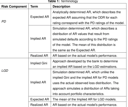
Table 1: Terminology

Risk Component Term Description

PD

Expected AR

Analytically determined AR, which describes the

expected AR assuming that the ODR for each

rating correspond with the PD ratings of the model.

Implied AR

Simulation determined AR, which describes a

distribution of AR values that result from

simulated defaults according to the PD ratings

of the model. The mean of this distribution is

the same as the Expected AR.

Realized AR AR based on the actual model’s performance.

LGD

Implied Gini Approach developed by the bank to determine an implied AR based on the LGD estimations.

Implied AR

Simulation determined AR, which unlike the

implied Gini and the implied AR for PD models

uses the actual observed loss distribution. The

approach simulates a distribution of ARs taking

into account portfolio characteristics.

Expected AR The mean of the Implied AR for LGD models.

Realized AR AR based on the actual model’s performance.

(8)

MANAGEMENT SUMMARY viii

In this study we attempt to find a systematic approach to set indicative benchmark values for the discriminatory power of an LGD model measured via theAccuracy Ratio(AR), which is a summary statistic for the discriminatory power of a classification model. LGD models are relatively new compared to PD models, but the last years have seen a significant num-ber of papers discussing the LGD model. Unfortunately, there is not yet an approach which indicates whether a model’s performance is sufficient in terms of discriminatory power. For these reasons the bank found it difficult determining what a sufficient level of discriminatory power for an LGD model is. Currently, they have set the threshold values fixed for each portfolio measured via the AR.

Various approaches to measure discriminatory power for LGD models exist and some are addressed in this thesis. Our investigation primarily focuses on the AR, which is also known as the Gini at the bank or Powerstat. The main reason to focus on the AR is that the bank uses this technique primarily to assess the discriminatory power of LGD models.

Implied Gini

As the bank felt that a threshold on discriminatory power that is the same for LGD models re-gardless of the underlying portfolio are not appropriate, it started a project which was aimed to find the AR that was implied by the LGD model. Initial research by the bank showed that the score of the AR is heavily dependent on the underlying product class for which the LGD model has been built. In order to find the potential discriminatory power of a model, the bank has developed the implied Gini coefficient. This approach was intended to indicate how well a model in potential can discriminate between the size of potential losses of debt instruments.

The idea of the implied Gini followed from a similar approach that has been developed for PD models, which indicated an expected AR if the PD model performed to its function. However, unlike the approach of the implied AR for the PD models the implied Gini for LGD models relies on a significant number of assumptions. We critically assessed these assumptions and found that the approach could not be generalized for four portfolios that were available for our investigation. Hence, based on our test results we conclude that the implied Gini is in its current form not valid. Adjusting the approach is not a possibility given the current available data and due to some critical assumptions that do not hold true.

Influencing Factors and Alternative Approach

(9)

In order to set these indicative benchmarks that depend on the portfolio characteristics we developed theimplied AR, which is a simulation driven approach that uses actual loss distri-bution instead of the estimations.1 For the development of an alternative approach we had to make choices due to the limit availability of data and cope with the current data quality. For the development of the alternative approach we limited ourselves by using the AR as a summary statistic. The main reasons for this choice are that for other summary statistics similar questions remain (e.g. ”what are acceptable values?”), and that the usage of the AR is common practice at the bank (and industry).

Within the process of developing an alternative approach we had to cope with several issues that cannot be solved due to the lack of data availability. Only the estimated LGD and the corresponding losses were available with some overall information concerning the portfolio, such as the historical cure rate. Therefore, we had to make choices, which can be consid-ered to be non-optimal. We argue, however, that regardless of this limitation, we can still proof that the current review approach of the bank can be improved by taking into account different portfolio characteristics. The alternative approach for the implied Gini we developed in this research still indicates that setting the same fixed threshold value for each portfolio is unnecessary penalizing particular portfolios. Our approach gives more insight in realistic AR values for specific portfolios compared to the current situation.

We acknowledge that the approach of the implied AR still relies on some basic assumptions that cannot be tested due to the lack of data or due to data quality. However, if more data becomes available or the data quality improves it could be the case that some assumptions are not necessary any more (e.g. such as the randomness of cure or fraud). The approach also relies primarily on quantitatively measurable factors that influence the AR. There might be, however, qualitative factors that indicate that it is more difficult for some portfolios to achieve higher levels of discriminatory power than others. In our research we found it diffi-cult to objectively pinpoint these factors as they are in our opinion very context dependent. Nevertheless, we think that the implied AR helps with the understanding of what (quantita-tively) drives the AR for LGD models and therefore helps to set up indicative benchmarks for discriminatory power measured via the AR.

1

(10)

(11)

Preface

Every student Industrial Engineering and Management at the University of Twente completes his MSc. degree with a graduation project either carried out internally at the university or ex-ternally at a company or an institution. I have chosen to conduct the final stage of my study program externally and I would like to thank the Rabobank for granting me this opportunity.

The project started in the summer of 2016 and over the course of the project many people helped me in getting to know the Rabobank, exchanged thoughts on the project or provided me with other valuable resources, which helped to write this thesis. I would like to especially thank to my supervisor Floris Bikker for guiding me through this process. I would also like to thank the members of the Risk Management team at the Rabobank, who were always available to help me with data issues or provide me with feedback on the project. Finally, I would like to thank Reinoud Joosten and Berend Roorda for providing feedback and new ideas.

Chris Sproates

(12)

(13)

List of Figures

1.1 Research Approach. . . 5

2.1 The Basel II framework as drafted by BCBS (2006). . . 9

2.2 Probability density function of losses (BCBS, 2005). . . 11

2.3 Validation methodology as drafted by BCBS (2005). . . 15

2.4 Examples of scatter plots for LGD data. . . 17

2.5 Example of a box-and-whisker plot. . . 17

2.6 Example of a CAP Curve. . . 23

2.7 Surfaces for AR. . . 23

2.8 Possible distributions for rating scores as found in BCBS (2005). . . 24

2.9 Example of an ROC Curve. . . 26

2.10 Surfaces for the AUC. . . 26

2.11 Example of an LC curve. . . 27

3.1 The histogram of resulting ARs for the development sample. . . 34

3.2 The histogram of resulting ARs for the validation sample. . . 34

4.1 Examples of different beta distributions (1). . . 40

4.2 Examples of different beta distributions (2). . . 41

5.1 Factors influencing the AR. . . 50

5.2 Impact of cures on the AR. . . 52

5.3 Distribution of all simulated ARs (example of Portfolio A). . . 54

5.4 Test results for experiment: 2PC-2 of Portfolio A. . . 58

(16)

List of Tables

1 Terminology . . . vii

2.1 Factors that impact the LGD score. . . 13

2.2 Six-point scale for LGD buckets as found in Cantoret al. (2006). . . 18

2.3 Example of a confusion matrix (count-based) . . . 19

2.4 Weights for the MAD as found in Liet al. (2009) . . . 20

2.5 Example of a confusion matrix (count-based) . . . 21

2.6 Example data for determining the Gini of a PD model. . . 22

2.7 Coordinates Perfect Model CAP curve. . . 23

2.8 Coordinates Rating Model CAP curve. . . 23

2.9 Example data for determining the ROC of a PD model. . . 26

2.10 Overview of techniques for measuring discriminatory power in this study. . . . 30

3.1 Assigned debtors per rating and sample. . . 34

3.2 Assigned debtors per rating and sample. . . 34

3.3 Implied AR for different calibrations. . . 35

5.1 Implied AR of the portfolios. . . 55

5.2 Implied AR of the structural LGD model. . . 55

5.3 Experiments for effect of different cure rates on the AR. . . 56

5.4 Test results for multiple cure rates in an LGD model (extreme cases). . . 57

5.5 Test results for multiple cure rates in an LGD model (random assignment). . . 58

5.6 Example data for the influence of the variance of a portfolio on the AR. . . 59

5.7 Test results for various fraud rates. . . 60

(17)

List of Acronyms

AR Accuracy Ratio

AUC Area Under the Curve

AUROC Area Under the Receiver Operating Characteristic

BCBS Basel Committee on Banking Supervision

BIS Bank of International Settlements

CEBS Committee of European Banking Supervisors

CAP Cumulative Accuracy Ratio

DNB De Nederlandse Bank

EAD Exposure at Default

EBA European Banking Authority

EL Expected Losses

FAR False Alarm Rate

GBR Generalized Beta Regression

GDP Gross Domestic Product

Gini Gini Coefficient

HR Hit Rate

IRB Internal Ratings-Based

LC Loss Capture

LGD Loss Given Default

LGL Loss Given Loss

LR Loss Rate

M Effective Maturity

MAD Mean Absolute Deviation

MAE Mean Absolute Error

(18)

LIST OF ACRONYMS xviii

MLE Maximum Likelihood Estimation

MOM Method of Moments

MSE Mean Square Error

ODR Observed Default Rate

PD Probability of Default

RAROC Risk-Adjusted Return on Capital

ROC Receiver Operating Characteristic

RR Recovery Rate

RWA Risk-Weighted Asset

SA Standardized Approach

SME Small or Medium Enterprises

(19)

Chapter 1 Introduction

In 2004 the Bank of International Settlements (BIS) published Basel II, which is the inter-national standard for the amount of capital that banks need to hold in reserve to deal with current and potential financial and operational risks (Persaud & Saurina, 2008).2 Part of this framework are the estimates of risk components for determining the amount of capital required for a given exposure. Subject to certain minimum conditions and disclosure require-ments, some banks have received supervisory approval to use the Internal Ratings-Based (IRB) approach for determining their own internal risk components (BCBS, 2006). Following from the framework of Basel II the risk components include the following measures:

1. Probability of default (PD).

2. Loss given default (LGD).

3. Exposure at default (EAD).

4. Effective maturity (M).

In the credit risk literature significant attention has been devoted to the estimation of the PD measurement, while much less attention has been devoted to the LGD measurements (Caouette et al., 2008). LGD is defined as the credit that is lost by a financial institution in the case a debtor defaults, expressed as a fraction of the exposure at default (Bastos, 2010). The accuracy of the LGD estimations are essential for computing economic capital and potential credit losses (Gupton, 2005). If a financial institution has accurate estimates of the risk components and models with adequate discriminatory power, it would mean in principal that a financial institution could gain a competitive advantage over its competitors as it is better in separating the ‘bad’ instruments from the ‘good’. Therefore, it is necessary that a financial institution is capable to estimate and validate the risk models used for finding the risk measures properly.

In order to determine the discriminatory power of an LGD model Rabobank uses the Gini coefficient (Gini), which is also known as the Accuracy Ratio (AR) or PowerStat. The term AR will be used in the remainder of this thesis as it used more frequently in literature. Pre-vious research by the bank has indicated that the AR is an adequate measure to determine the discriminatory power of an LGD model. In this thesis, however, some critical side notes on the AR are given. The AR is described in Chapter 2.

2_{Additional regulations were added in Basel III.}

(20)

CHAPTER 1. INTRODUCTION 2

Measuring the discriminatory power of LGD models is relatively new compared to PD mod-els, which means that there is less experience in modelling those type of models. In recent years more research and best practices on LGD models emerged, but compared to PD models it is still significantly less. The relative inexperience in modelling the LGD model component has made it difficult to determine what a sufficient level of discriminatory power for an LGD model is compared to PD models.

Hence, the bank started a project to find indicative benchmarks for discriminatory power measured via the AR. Initial research showed that the score of the AR is heavily dependent on the underlying product class for which the LGD model has been built. In order to find the maximum attainable discriminatory power of a model, the bank has developed the so-calledimplied Gini coefficient. This approach was intended to indicate how well a model in potential can discriminate between the size of potential losses of debt instruments. It was intended to derive an indicative benchmark for discriminatory power from the implied Gini. The realized AR (via historical data) indicates the actual performance of a model on discrim-inatory power. If the realized AR is above the threshold derived via the implied Gini, then the model is perceived to have performed to its abilities according to the bank. The formal definition of the implied Gini that has been developed by the bank is presented in Chapter 3.

In this study we review the approach developed by the bank and recommend whether it can be used in its current form. We review the underlying assumptions on the implied Gini made by the bank and research alternative methods for setting the target value for the discrimina-tory power of LGD models based on the AR. We provide recommendations on which method should be used for setting a target value of the discriminatory power. This chapter has the following outline:

Section 1.1: We describe the background and motivation of this study.

Section 1.2: We present the research objective.

Section 1.3: We describe the research approach.

Section 1.4: We cover the research questions, which are to be answered in this thesis.

Section 1.5: We present the outline of the thesis.

1.1 Credit Risk at Rabobank

The Rabobank is an international financial services provider operating on the basis of coop-erative principles (Rabobank Group, 2015). It offers services such as retail banking, whole-sale banking and private banking. Furthermore, in 2015 it was the second largest bank in the Netherlands measured in total assets (TheBanks.eu, 2016). One of the core activities of the Rabobank is providing savings and borrowing services, which leads to a private sector loan portfolio (outstanding credit) of EUR 426,157 million euro compared to the total assets of EUR 670,373 million (Rabobank Group, 2015).

(21)

expectation will not be met”. In order to cope with the risk that a debtor is not able to meet his financial obligations the bank has to hold capital. For this form of risk mitigation banks are required to hold mandatory regulatory capital and in addition they can hold economic capital, which is an internally computed measurement by banks to manage their risks. As a result of these regulations in 2015 the Rabobank reserved EUR 17.0 billion of which 86% is for credit and transfer risk. The bank computed their economic capital to be EUR 26.7 billion of which 54% attributes to credit and transfer risk.

In accordance with the regulation, the bank uses the advanced IRB approach to calculate its regulatory capital for credit risk for basically the whole loan portfolio. In accordance with the supervisor the Standard Approach (SA) is used for some portfolios with relatively limited exposure and a few small foreign portfolios as the advanced IRB is not suited (Rabobank Group, 2015). The difference between the two approaches is the way in which the risk-weighted assets (RWAs) are computed, which is the input variable for computing the first pillar capital requirements of Basel II. As Hull (2012) describes, the total required capital is computed via Eq. (1.1).

Total Capital = 0.08·(credit risk RWA + market risk RWA + operational risk RWA) (1.1)

The current SA prescribes that external credit ratings are used as input in order to determine the (credit risk) RWA, while for the advanced IRB the banks supply their own estimates of the PD, LGD, EAD, and M to estimate the RWA (BCBS, 2015; Hull, 2012). In Chapter 2 a detailed overview of the Basel II framework and its risk components (especially the LGD component) is given. We describe how these risk components are used to compute the RWA via the (advanced) IRB approach.

As the bank is allowed to estimate its own risk components for a large part of its portfolio (under compliance of supervisory standards) it is important that the estimates are accurate. Underestimation of the risk components means that the mitigation of risk is not sufficient and extreme losses on the loan portfolio are not covered. Overestimation of risk is also un-desired as the bank then holds additional capital, which does not yield a return.

It is important that the estimates of a risk model are accurate, but a model can be accurate in estimating the total portfolio losses without correctly estimating the risk components on an individual (observation) level. If a risk model is not able to differentiate between the ’good’ and ’bad’ loans, it should be considered as invalid because clients with an actual high credit risk will have to post relatively less collateral compared to clients that are in reality less risky. Therefore, it is not only important to validate the estimates of the risk models, but also the discriminatory power of the risk models. Kraftet al. (2002) indicates that there is no formal definition for the discriminatory power of risk models. For that reason, study follows the def-inition given by Prorokowski (2016), namely ”the ability to differentiate between defaults and non-defaults, or high and low losses”. For LGD models the discriminatory power would then be the ability to differentiate between the severity of losses.

(22)

It has developed the implied Gini to create a target value for the assessment. We review the original approach that has been developed by the bank and we suggest an alternative approach to set indicative benchmarks for discriminatory power via the AR.

1.2 Research Objective

The objective of this study is to develop an approach to set indicative benchmarks for mea-suring discriminatory power via the AR. The general method should provide guidance in setting a target value for the discriminatory power of an LGD model. The indicative bench-marks should give the bank insight in the performance of the model on discriminatory power. It helps the bank in deciding, whether the model can be accepted or should be redeveloped. Part of this study is the review of the implied Gini developed by the bank. The method has been developed on the basis of assumptions that not have been validated or proven to be correct prior to this study. Before the implied Gini can be applied for model validation, it is required that these assumptions are investigated in-depth and tested on their validity. The first part of this study focusses on the validity of the current method.

XXXXXXXXXXXXXXXXXXXXXXXXXXXXXXXXXXXXXXXXXXXXXXXXXXXXXXXXXX XXXXXXXXXXXXXXXXXXXXXXXXXXXXXXXXXXXXXXXXXXXXXXXXXXXXXXXXXX XXXXXXXXXXXXXXXXXXXXXXXXXXXXXXXXXXXXXXXXXXXXXXXXXXXXXXXXXX XXXXXXXXXXXXXXXXXXXXXXXXXXXXXXXXXXXXXXXXXXXXXXXXXXXXXXXXXX XXXXXXXXXXXXXXXXXXXXXXXXXXXXXXXXXXXXXXXXXXXXXXXXXXXXXXXXXX XXXXXXXXXXXXXXXXXXXXXXXXXXXXXXXXXXXXXXXXXXXXXXXXXXXXXXXXXX

As the goal of this study is to develop a new general approach to set indicative benchmark values for LGD models this study can be described as theory oriented research following the design methodology for setting up a research project by Verschuren & Doorewaard (2007). They distinguish two types of theory oriented research, namely theory developing and the-ory testing. This study contains both types as we review the approach developed by the bank (implied Gini), which is theory testing oriented, while we also develop a new approach for setting indicative benchmarks for LGD models, which is theory developing oriented.

(Goal) Develop a systematic approach to set indicative benchmark values for the discrimi-natory power of an LGD model measured via the AR.

1.3 Research Approach

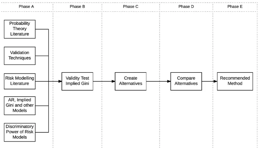
Before the actual study can start, it is important that all stakeholders agree on what the scope and content of the research is. A good approach to get an agreement and to man-age expectations is making use of a research model, which allows every stakeholder to get a quick overview of the contents of the study. Resulting from the contextual framework from which the study subject originates (see Section 1.1) and the research objective (see Section 1.2) it is possible to derive a research approach. This model is visualised in Fig. 1.1.

(23)

[image:23.595.108.524.93.329.2]

Figure 1.1: Research Approach.

and possible ideas to develop new approaches. Besides the theoretical framework, it is im-portant to create a clear description of the method including all its assumptions, which is the subject of the validation process. Based on the test results following from the application of the validation techniques and the theoretical framework, it is possible to determine whether the current method of the implied Gini is valid for measuring the discriminatory power of a LGD model (Phase B). The results of Phase B determine, whether the implied Gini is taken into account as a valid alternative for setting indicative benchmarks for measuring the dis-criminatory power of an LGD model. In Phase C different approaches for setting indicative benchmarks are examined and developed. For all the valid methods the (dis-)advantages are compared (Phase D), which after consideration leads to a recommended method (Phase E).

1.4 Research Questions

From the research objective and model it is possible to derive the questions that this study has to answer. The main research question of this study is:

(Main) Which factors should the bank take into account to determine the indicative bench-marks for the discriminatory power of an LGD model?

To answer this question, the working of LGD models in general and the process of validation need to be described first in order to create a contextual framework and a general under-standing. Once the framework has been established and the challenges concerning LGDs have been described, methods for assessing discriminatory power of an LGD model are discussed.

(1.1) Which methods are available to assess the discriminatory power of an LGD model?

(24)

(1.3) What are the differences between a PD model and an LGD model for measuring and benchmarking discriminatory power?

If a general overview is created of possible methods to assess discriminatory power the current workings of the implied Gini and its assumptions can be explored in-depth. The current method of the implied Gini is based on the research done by the bank.

(2.1) How does the current method of the implied Gini coefficient work?

(2.2) Which assumptions have been made for developing the implied Gini?

After the explanation of the implied Gini method, it is required to validate the assumptions that have been made.

(3) Do the assumptions for the implied Gini hold?

If the method is valid, it can be used to get more insight in establishing the benchmark for backtesting the discriminatory power of an LGD model via the AR. Regardless of whether the implied Gini is valid or not, it still does not provide a solution to setting an actual threshold value for the back-test of discriminatory power for an LGD model. The second part of the study focusses on what drives the AR score of an LGD model and when an LGD model is considered to be ’good’.

(4) Which factors impact the AR score of an LGD model?

Based on the answers on all the research questions possible approaches for setting in-dicative benchmarks of an LGD model are developed. After the comparison of the possible methods a suggested systematic approach for establishing a benchmark value is presented.

1.5 Outline

The remaining part of the thesis has the following structure:

Chapter 2: We provide an in-depth analysis of LGD models, the discriminatory power and the methods to assess this attribute. The findings from literature are put into context of this study. We conclude this chapter with the answer to the first sub-questions.

Chapter 3: We explain the current method for determining the implied Gini coefficient. Furthermore, we describe the main differences between PD and LGD models that are relevant for measuring discriminatory power as there exist a similar concept of an implied AR value for PD models. The chapter concludes with the answers to sub-questions 2.1-2.2.

(25)

Chapter 5: We investigate LGD models more in-depth and determine which characteris-tics impact the AR score of an LGD model. Within this chapter we develop an alternative approach for establishing a threshold value based on the AR given the limitations on data in practice. We conclude with the answers to sub-question 4.

Chapter 6: We propose an approach to set indicative benchmarks for testing the discrimi-natory power of an LGD model based upon the approach we develop in Chap-ter 5.

(26)

Chapter 2 LGD Models and Their

Discriminatory Power

Before the method of the implied Gini is discussed in-depth, it is necessary to establish a common understanding of risk models in general, and the challenges for modelling LGDs. Therefore, this chapter firstly elucidates the framework of Basel II for the (advanced) IRB approach. Secondly, an overview of processes and common practices in modelling and validating LGD models is given. The overview is based on findings from literature as well as internal documents and practices at the Rabobank. Finally, approaches for measuring the discriminatory power as well as the method for determining the AR of an LGD model is discussed.

The terminology, used in the internal documentation at the Rabobank, is adopted in this the-sis as well for conthe-sistency reasons. The term LGD refers to the loss given defaultestimate, which is expressed as a percentage of the Exposure at Default (EAD). The actualobserved

loss has the term loss rate (LR) and is expressed as a percentage of the observed EAD. The LGD and LR term are sometimes also called estimated LGD and the realized LGD. This documentation will use the terms from the latest policy documentation, hence LGD and LR are used.

This chapter has the following outline:

Section 2.1: We discuss the Basel II Framework for the (advanced) IRB approach.

Section 2.2: We illustrate the complexity of modelling of LGD models as a lot of factors have to be taken into account.

Section 2.3: We describe a high level overview of the validation process and approaches for estimating LGDs.

Section 2.4 We describe the general structure of risk models used at the bank.

Section 2.5: We give an overview of techniques for assessing the performance of LGD model.

Section 2.6: We give an overview of techniques for assessing the discriminatory power.

Section 2.7: We describe the internal guidelines and processes of LGD validation at the bank.

Section 2.8: We provide answers to the first sub-questions.

(27)

CHAPTER 2. LGD MODELS AND THEIR DISCRIMINATORY POWER 9

2.1 The Basel II Framework for the (advanced) IRB Approach

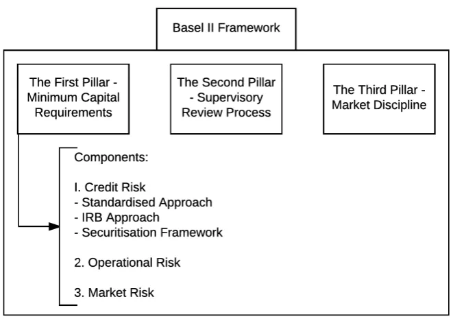
[image:27.595.147.478.252.486.2]

As discussed in the introduction, the BIS published in 2004 Basel II, which is i.a. a com-prehensive framework of standards on how to measure various risk components and forms the basis on the amount of regulatory capital a financial institution has to reserve in order to cope with various risks. This section will focus on the regulatory and economic capital that is kept for dealing with credit risk. This is part of the first pillar of Basel II (which in total consists of three different pillars). The first pillar of Basel II describes the conditions and guidelines for determining the minimum capital requirements. It differentiates between three forms of risk, namely credit, operational and market risk (BCBS, 2006). An overview of the structure of Basel II based on BIS documentation can be found in Fig. 2.1.

Figure 2.1:The Basel II framework as drafted by BCBS (2006).

Technically the IRB approach can be split up into two different approaches, namely the foun-dation IRB approach and the advanced IRB approach. The difference between the two approaches is that for the foundation approach the PD is estimated by internal models of a financial institution, but the LGD and EAD are determined on fixed values provided by the supervisor. In the advanced approach the bank uses internal models to estimate the PD, LGD and EAD. M is computed in the same way for both approaches, if M plays a role in the portfolio (DNB, 2007). If a bank has received supervisory approval, it may use the advanced IRB approach. Using the IRB approach has benefits for the regulators as well as the finan-cial institutions. Finanfinan-cial institutions are incentivised to take on customers with low scores for PDs and LGDs as they result in lower risk weightings and therefore lower capital reserve requirements. It results in some form of self-surveillance, which also decreases the costs of regulation and potential legal battles with banks (Balin, 2008). As this study primarily focuses on LGD models we only the advanced IRB Approach is discussed in detail.

As is described in the BIS documentation3the following equations are to be used to derive the RWA, which is used as input for calculating the minimum required capital via Eq. (1.1).

3

(28)

Please note that the PD and LGD are measured in percentages, and the EAD is measured as a currency in the BIS documentation. The PD value represents the probability that the loan will go into default within one year. The LGD is expressed as the fraction of the EAD that is lost if the loan goes into default (see Chapter 1). Thelnin Eq. 2.2 denotes a natural logarithm. N(x) in Eq. 2.3 denotes the cumulative distribution function of a standard normal random variable. G(z) denotes the inverse cumulative distribution function for a standard normal random variable (see BCBS, 2006).

R= 0.12·1−e

−50·PD

1−e−50 + 0.24·

1−1−e

−50·PD

1−e−50

(2.1)

b= (0.11852−0.05478·ln PD)2 (2.2)

(2.3) K = LGD·N (1−R)−50·G(PD) +

R 1−R

0.5

·G(0.9999)

!

−PD·LGD

!

·(1−1.5·b)−1·(1 + (M−2.5)·b)

RWA =K·12.5·EAD (2.4)

Eq. 2.1 - 2.4 illustrate how the RWA for credit risk is determined under the advanced IRB approach. The correlationRand maturity adjustmentbare input values among theLGD,PD

andM estimates for the computation of the capital requirementsK. The RWA is a function ofK and the EADestimate. There are some adjustments for specific asset classes, which are not treated in this study. For a complete overview see the documents published by the BIS (see References). The output of Eq. 2.4 is used as input for Eq. 1.1.

Economic capital is, as mentioned in Chapter 1, the internal estimate of the capital that is required to be held by a financial institution in order to cope with the risk it is taking. A more formal definition is that economic capital is the allocated capital a financial institution needs in order to absorb losses over one year with a certain confidence level (Hull, 2012). Regula-tory capital is, more or less, computed via one-size-fits-all rules created by the BCBS. Hull (2012) states that ”economic capital can be regarded as a ’currency’ for risk-taking within a financial institution”. He explains that a business unit is only allowed to take a certain risk when it has allocated the right amount of economic capital, and the profitability of the busi-ness unit is measured relative to the allocated economic capital. The latter is measured via the risk-adjusted return on capital (RAROC), which is not discussed further in this study as it lies beyond the scope of this research.

In Fig. 2.24 a typical density function for credit losses can be found, which describes the likelihood of losses of a certain magnitude (BCBS, 2005). Capital reserved to cope with risk is used to cover unexpected losses (UL). The confidence level depends on the credit rating a financial institution wishes to pursue. If a bank for instance wishes to maintain an AA credit rating, then their probability of default in one-year would be about 0.03%. This suggests the confidence level for the determination of the amount of economic capital should be set at 99.97% (Hull, 2012). For financial institutions the expected losses (EL) of credit are a

4

(29)

useful measure as well, as that indicates the amount it should hold in reserve from fees and interest revenues to absorb the losses that are likely to occur over the course of a year thus it is an important input factor for loan pricing decisions (Herring, 1999).

Figure 2.2: Probability density function of losses (BCBS, 2005).

The expected loss from defaults is determined via the risk components PD, LGD and EAD, which are estimated for each counterpartyi. Hull (2012) shows that the total expected losses from defaults are then:

X

i

EADi·LGDi·PDi (2.5)

The LGD is related to the recovery rate (RR), which is the amount that is recovered from a defaulted credit. It has the following definition (expressed in percentages):

RR = 1−LGD (2.6)

From Basel II we conclude that it is crucial to have accurate estimations for the risk compo-nents to determine the necessary capital required for absorbing the potential risks. In the upcoming sections more attention will be paid to which factors affect the LGD and how it is validated.

2.2 Factors Affecting the LGD Scores

The LGD becomes relevant if a particular obligor has gone into default, which will start the process of trying to (partly) recover or salvage the outstanding credit. Default for a particular obligor has been defined by the BCBS (2006) if one or both of the following conditions has been met:

• The obligor is unlikely to pay its credit obligations to the financial institute in full from the creditors perspective, without recourse by the bank to actions.

• The obligor is past due more than 90 days on any material credit obligation to the banking group.

(30)

on credit obligations), but makes good on all their obligations in the next period. If a bank ignores such events and does not record this as recoveries in the bank’s loss data, it might underestimate the RR on loans (Schuermann, 2004). This can be considered to be a cure, which is the event that a loan, which is declared to be in default, recovers and no loss is observed. It should be noted that an LGD of 0% does not explicitly mean that the default cured. Baesens & Van Gestel (2009) illustrate a similar issue of underestimating scores via technical defaults, which they define as the event that a counterparty fails to pay timely due to reasons that are not related to the financial position of the borrower. If a bank classifies the technical default as a default (from the definition of Basel II), it will typically result in a higher number of registered defaults, but in general a lower LR value.

In general, the LGD following from a default is a ratio of the losses to the EAD. One would think that it is not possible to have losses that are larger than the EAD, but it might occur in practice that the actual LGD is larger than 100%. There are namely various sources of a loss, which Schuermann (2004) distinguishes into three types:

• The loss of the principal, which is the original amount that has been lent (e.g., book value).

• The carrying cost of non-performing loans (e.g., interest income that cannot be re-trieved).

• Workout expenses, which are e.g. costs made to collect the loan or collateral, or legal costs.

Due to for instance high workout costs, it might occur that the LR is larger than the actual EAD, resulting in an LR greater than 100%. Besides the workout expenses in case of a de-fault, the seniority of the debt instrument and the posted collateral play important roles. The seniority determines the priority for all the creditors in the case value can be salvaged from a default. Collateral is a specific asset or property pledged to the creditor in the case of a de-fault and used to secure debt instruments. Empirical evidence suggests that the seniority of bonds is one of the driving forces behind an RR, as the mean recovery increases for higher levels of seniority (Altman & Kishore, 1996). As loans are generally senior to bonds, it is ex-pected that they will also provide higher RRs than bonds. Statistics resulting from Moody’s database of 1970 till 2003 imply that RRs for loans are typically higher (Schuermann, 2004). A similar correlation can be found between collateral and RR (Grunert & Weber, 2009).

Another factor that has been described by Altmanet al. (2005) is the negative correlation between the observed default rate (ODR, which is the actual number of defaults observed in a time period, and the RR (for corporate bonds): Higher aggregated levels of the ODR tend to coincide with lower RRs. Frye (2000) also indicates that in the US years that have a relatively high default rate, will result in a lower RR on average. The years that he indicated as the years with a high default rates (1990 and 1991) coincide with relatively low growth in gross domestic product (GDP), namely 1.9% and -0.1% on an annual basis (The World Bank, 2016). The other years in Frye’s data set had a minimum growth of 2.7%. This relation could imply that in recessions or times of slow economic growth the RRs are lower than in times of expansions.

(31)

However, Qi & Zhao (2013) suggest that the impact of the industry and macroeconomic variables on the LGD vary with the sample, model specification and modelling technique used. Their research suggested that the debt structure of a firm should be considered for modelling the RR.

A difference in RRs between countries is observed by Davydenko & Franks (2008). Their research suggested i.a. that the local bankruptcy code affects the RR, as in countries that are perceived to be debtor-friendly (e.g., France) the RR is considerably lower than in more creditor-friendly countries. They state that the influence of the bankruptcy code is the great-est in explaining the differences between the recoveries. Furthermore, they state that the bankruptcy codes also result in different lending and reorganization practices as e.g. the posted collateral in France is higher than in Germany and U.K., which are perceived to be more creditor-friendly.

The brief overview from the literature illustrates some of the difficulties to model LGDs. A lot of variables need to be taken into account in order to estimate a LGD correctly. Different portfolios have their own specific LGD models. Table 1 includes, but is not limited to, factors that influence the values of an LGD. Additional explanatory factors for LGD estimation can be found in Peters, C. (2011).

Table 2.1: Factors that impact the LGD score.

Factor Literature

Definition and Recording of Defaults Schuermann (2004), Baesens & van Gestel (2009)

Debt Type, Seniority and Collateral Altman & Kishore (1996), Schuermann (2004), Grunert & Weber (2009)

Debt Structure Qi & Zhao (2013)

Default Rates and Macroeconomic Develop-ments

Frye (2000), Schuermann (2004), Altmanet al. (2005)

Type of Industry Altman & Kishore (1996), Schuermann (2004), Acharyaet al. (2007)

Bankruptcy Code (in Country) Davydenko & Franks (2008)

2.3 LGD Modelling and Validation

(32)

Approaches for LGD Estimation

In order to estimate the LGD various techniques (or combinations) can be used. There are four approaches described by the Committee of European Banking Supervisors (CEBS)5

(2006) to estimate an LGD, which are the following:

Workout LGD calculates the (discounted) cash flows resulting from a workout and/or collections process.

Market LGD determines the LGD estimations on the basis of the market prices of defaulted obligations.

Implied Market LGD is similar to the Market LGD, but estimates the LGD from non-defaulted loans, bonds or credit default instruments. The im-plied market LGD is derived via a theoretical asset pricing model (Schuermann, 2004).

Implied Historical LGD is a technique that derives the LGD from the realised losses on exposures within a loan portfolio and PD estimations. CEBS (2006) allows this technique only for the Retail exposure class (e.g. loans made to individuals such as mortgages).

As CEBS (2006) points out, the supervisors do not require that a specific technique is used for the LGD estimations. Nevertheless, financial institutions will need to demonstrate that the assumptions underlying their models are justified and that the approach is appropriate for the specific portfolios to which it is applied as the results might be different per approach. For example, the realized workout LGD usually takes some time to be computed as it uses the discounted values of actual cash and assets after a default has been settled, while the market LGD is easy to observe from actual market prices. Renault & Scaillet (2004) state that the market LGD has its drawbacks.6 They state i.a. that the trading price recovery tends to have lower means compared to the ultimate recovery. An advantage, however, is that it is not required to choose a specific discount rate and because the market LGD is derived from actual market prices an investor can determine the RR if he liquidates his position im-mediately. For the estimation of an LGD one should carefully assess the drawbacks and advantages of the different approaches. The choice is also dependent on the type of port-folio, as not all approaches can be used for some portfolios. For example, not all types of portfolios have market data to derive RRs.

LGD Validation Methodology

Once an approach for the LGD estimation has been chosen and a model has been devel-oped the process of validation may begin. An LGD model should be reviewed periodically as it is important to see whether the LGD model is still accurate. This is done by validating the model by i.a. backtesting and benchmarking the risk components.

The BCBS (2005) notes that the use of statistical tests for backtesting may be difficult as the data from financial institutions may be constrained. The reason behind this might be

5_{Their tasks and responsibilities have been taken over by the European Banking Authority (EBA) as from}

2011.

6

(33)

[image:33.595.110.516.103.339.2]

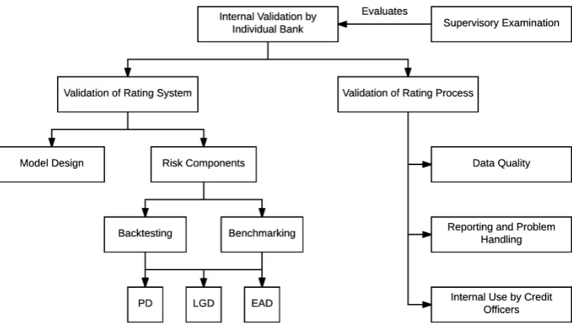
Figure 2.3:Validation methodology as drafted by BCBS (2005).

the low number of defaults in a portfolio or low internal data quality. Initiatives have been started according to the BCBS (2005) to build consistent data sets. There is an emphasis on the validation of LGDs in the studies conducted by the BCBS, as i.a. the capital charges are quite sensitive to the LGD (see Eq. 2.1-2.4). A high level overview of the validation methodology drafted by the BCBS (2005) can be found in Fig. 2.3.

A practical framework for the validation of an LGD model is described by Li et al. (2009). They define three specific performance goals, which are of interest for the credit risk man-ager. The goals are as follows:

• Good performance on the rank-order of different LGD estimations (discriminatory power).

• Accurate predictions of the LR (calibration).

• Accurate prediction of the total observed portfolios loss amounts, which assumes that the PD model correctly distinguishes between defaulters and non-defaulters.

Lotermanet al. (2012) point out that a good ranking does not imply that the calibration is good, but on the other hand if the calibration is good it always implies that the discriminatory power is good as well. After the (re-)validation process Liet al. (2009) distinguishes three possible outcomes that may result from the assessment, namely:

• LGD model is a reasonable reflection of the current portfolio and performs well enough— no adjustments to its current form are required.

(34)

• LGD model is significantly different from the original specification or a previous revali-dation process, and is not likely to meet its expected performance level—a redevelop-ment is required.

In order to validate the risk models a variety of tools and metrics are available to recognize under-performing LGDs. As this study intends to find a valid method to establish a target value for the discriminatory power which can be used as a benchmark in the validation process an overview of frequently used techniques are presented in Section 2.4. The main focus is on the assessment of the discriminatory power of LGD models.

2.4 Risk Model Structure

XXXXXXXXXXXXXXXXXXXXXXXXXXXXXXXXXXXXXXXXXXXXXXXXXXXXXXXXXX XXXXXXXXXXXXXXXXXXXXXXXXXXXXXXXXXXXXXXXXXXXXXXXXXXXXXXXXXX XXXXXXXXXXXXXXXXXXXXXXXXXXXXXXXXXXXXXXXXXXXXXXXXXXXXXXXXXX XXXXXXXXXXXXXXXXXXXXXXXXXXXXXXXXXXXXXXXXXXXXXXXXXXXXXXXXXX XXXXXXXXXXXXXXXXXXXXXXXXXXXXXXXXXXXXXXXXXXXXXXXXXXXXXXXXXX XXXXXXXXXXXXXXXXXXXXXXXXXXXXXXXXXXXXXXXXXXXXXXXXXXXXXXXXXX

2.5 General Techniques to Get Insight in the Performance of

LGD Models

Before techniques for assessing the discriminatory power of an LGD model is described, some general techniques to get insight in the performance of an LGD model are introduced. First possible techniques to visualise the performance of an LGD model are described. After the description of these visualisation techniques error measures are introduced, which indi-cates the performance of the model on accuracy and calibration. In Section 2.6 techniques for assessing discriminatory power are discussed, which is the main focus of this thesis.

Summary Plots

According to Liet al. (2009) one of the first plots that has to be examined when validating an LGD is the scatter plot of the LGD versus the LR. This helps to provide evidence whether the estimations of the model correspond with the actual LRs. A good model should be able to provide a scatter plot with points concentrated around the diagonal. A perfect model would be able to provide a line through the origin, while having a 45◦angle. Fig. 2.4 provides a simplified example of the difference between the scatter plot of a ‘bad’ LGD model and a ‘good’ LGD model.

In order to see whether the assumed loss distribution corresponds with the realized loss distribution histograms allow a good visual comparison between the two distributions. To ac-tually see whether the LGDs and LRs originate from the same distribution various statistical tests are at the credit risk managers’ disposal (e.g., two-sample Kolmogorov-Smirnov test). These techniques are discussed in-depth in Chapter 4.

(35)

Figure 2.4:Examples of scatter plots for LGD data.

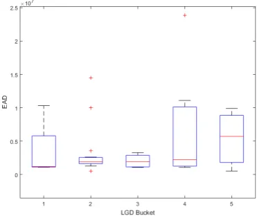
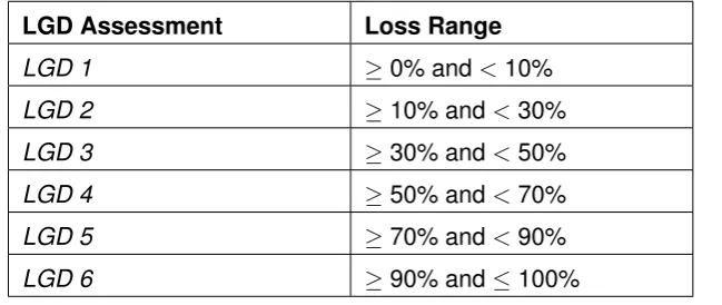
[image:35.595.217.403.526.682.2]

to grasp the characteristics of the EAD distribution as a histogram is often not enough. This graphical approach is simply a representation of the median and the quartiles (the box) and possible outliers (whiskers) for a particular data set. If this technique is used for getting in-sight in the performance of an LGD model then the box-and-whisker plot can show how the EADs of a portfolio are distributed against LGD estimations. Appendix A contains random sample data of the EAD and LGD for 50 debtors in a portfolio. In order to construct the box-and-whisker plot the data set is separated in 6 buckets based on the LGD estimation. The buckets ranges are based on the ranges suggested by Cantoret al. (2006) as found in Table 2.2. The sixth bucket is empty in our example (no estimations larger than 90%). For the remaining buckets a box-and-whisker plot is made on the basis of the EADs contained in a bucket. Fig. 2.5 shows the resulting box-and-whisker plot for the example data found in Appendix A. For this data set the plot shows that the EADs have a large range in most buckets and the spread also varies between the buckets, which is something to be taken into account for the validation process.

(36)

Error Measures

Summary plots can be used to get a quick overview of the LGD models performance, but in order to quantify the LGD models performance error measures can be used. One approach suggested by Liet al. (2009) is the use of confusion matrices. These type of matrices are used to check how a classifier model performs. In order to construct the confusion matrix for an LGD model, it is required to have the LGD estimations and realizations (the LR). Each LGD estimation is classified to its corresponding bucket (e.g. via the six-point scale as found in 2.2), and the same process is followed for the realizations. We denote for each instance its corresponding estimated LGD asLGDEST_p and its LR asLGDREA_p forp= 1,2, ..., nwithn

instances. We denote the total number of classes (e.g. the buckets as found in 2.2) askand each possible assignment forLGDREA_p asi = 1,2, ..., k and forLGDEST_p asj = 1,2, ..., k. Each bucket has a lower bound and upper bound, which determines whether an estimation or realization as assigned to the bucket. These bounds are denoted by LB and UB. Via Eq. (4.10) it is possible to determine the corresponding buckets for both the estimated and realized LGD.

cp,i,j =



 

 

1, if LBi ≤LGDREAp <UBi and LBj ≤LGDESTp <UBj

0, otherwise

(2.7)

If for each of the paired observations the corresponding classes or buckets are determined, then it is possible to compute the confusion matrix. The idea behind the confusion matrix is to count for each cell in the matrix the number of pairs within such a cell. The total number of pairs in a cell is denoted viaai,j and computed via Eq. (2.8).

ai,j = n

X

p=1

cp,i,j (2.8)

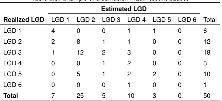
[image:36.595.155.480.611.748.2]

In Table 2.3 the confusion matrix for the sample data in Appendix A can be found (based on the buckets in Table 2.2). The diagonal of the matrix shows how many LGDs have been estimated in the correct bucket (i.e., they have been correctly classified). The other cells of the matrix show how many LGDs have been falsely classified. Take for example the cell (LGD 6, LGD 4), which has the value of 1. This particular instance has been estimated to be in Bucket 4 (50% till 70%). The realized LGD of this instance is, however, above 90% and therefore it actual ’class’ is Bucket 6.

Table 2.2: Six-point scale for LGD buckets as found in Cantoret al. (2006).

LGD Assessment Loss Range

LGD 1 ≥0% and<10%

LGD 2 ≥10% and<30%

LGD 3 ≥30% and<50%

LGD 4 ≥50% and<70%

LGD 5 ≥70% and<90%

(37)

[image:37.595.124.505.100.273.2]

Table 2.3: Example of a confusion matrix (count-based)

Estimated LGD

Realized LGD LGD 1 LGD 2 LGD 3 LGD 4 LGD 5 LGD 6 Total

LGD 1 4 0 0 1 1 0 6

LGD 2 2 8 1 1 0 0 12

LGD 3 1 12 2 3 0 0 18

LGD 4 0 0 1 2 0 0 3

LGD 5 0 5 1 2 2 0 10

LGD 6 0 0 0 1 0 0 1

Total 7 25 5 10 3 0 50

This approach is called ’count basis’ by Li et al. (2009). The other approaches they have described are intuitively the same, but might require more information such as EAD or ob-served losses values, which are defined respectively as the ’total EAD basis’ and ’obob-served loss basis’ approach. In the ’total EAD basis’ approach one sums the total EAD for each cell. If the observation in the cell (LGD 6, LGD 4) is again taken as an example, the value for that cell in the ’total EAD basis’ approach would bee11.100.000. This is 6.09 % of the total EAD for the whole portfolio (e182.400.000), while it only represents 2% of all the ob-servations (50). If the EADs are more or less equal in size the ’count-basis’ approach would be appropriate, but in our example (also indicated by the box-and-whisker plot in Fig. 2.5) the exposure at risk might be underestimated as some miss-classifications represent a large risk.

The ’observed loss basis’ approach uses the realized losses instead of the EAD. This ap-proach illustrates the impact of particular miss-classifications. The realized loss of the in-stance in the cell (LGD 6, LGD 4) is e10.989.000, which is 14.75% of the total losses (e74.488.650). The realized losses are obtained by multiplying the LR with the EAD. This shows that the impact of this miss-classification is quite severe in our example portfolio.

Liet al. (2009) argue that, besides the overview the confusion matrix gives of the model’s performance, there still is a need to capture the information contained by the confusion ma-trix in a single metric. This metric allows a comparison between LGD models. They suggest two metrics as a measurement, namely the ’percent matched’ and ’Mean Absolute Deviation (MAD)’. The metric percent matched indicates how many LGDs are correctly estimated to belong in the realized bucket. Looking to the confusion matrix in Table 2.3, this means that all the values on the diagonal are the correctly estimated values. The score on this metric is the sum of all the elements of the diagonal divided by the total number of elements in the data set. This is defined in Eq. 2.9 for which k is defined as the number of buckets (thus leading to ak-by-k confusion matrix),ai,j as a matrix cell (thusai,i is the element on

the diagonal), andn represents the total number of observations in the data set. In sample confusion matrix (see Table 2.3) 18 out of the 50 elements are on the diagonal, which leads to a performance score of 36%.

Percent Matched =

Pk

i=1ai,i

(38)

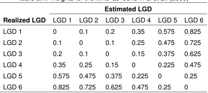
[image:38.595.142.486.233.388.2]

The other performance metric suggested by Li et al. (2009) is the ’Mean Absolute Error (MAE)’, which takes into account how ’bad’ the miss-classification was. They argue that a classification for a neighboring bucket can be considered as less severe than a classification of bucket that is further away from the actual realized bucket. For instance a classification in the cell (LGD1, LGD2) is ’less’ wrong than a classification in the cell (LGD1, LGD6). The standard ’percent matched’ approach does not take this into account. In order to take the ’severeness’ of a miss-classification into account they compute the absolute deviation between the buckets. In order to do so they have determined weights for each bucket, which can be found in Table 2.4. These weights can of course be set differently.

Table 2.4: Weights for the MAD as found in Liet al. (2009)

Estimated LGD

Realized LGD LGD 1 LGD 2 LGD 3 LGD 4 LGD 5 LGD 6

LGD 1 0 0.1 0.2 0.35 0.575 0.825

LGD 2 0.1 0 0.1 0.25 0.475 0.725

LGD 3 0.2 0.1 0 0.15 0.375 0.625

LGD 4 0.35 0.25 0.15 0 0.225 0.475

LGD 5 0.575 0.475 0.375 0.225 0 0.25

LGD 6 0.825 0.725 0.625 0.475 0.25 0

The absolute deviation is computed by multiplying the weight for each cell with the counted number in each cell as defined by Eq. 2.10. Thewi,j is the weight for the combination (i,j)

andai,j is the number of elements in each combination (i,j).

ADi,j =wi,j·ai,j (2.10)

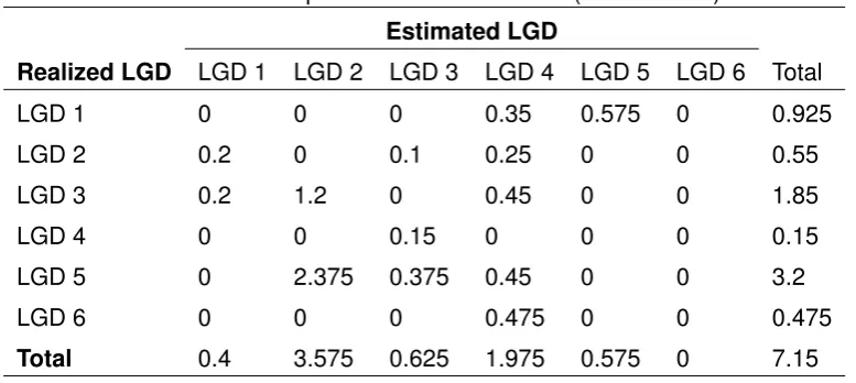
If the same weights used by Li et al. (2009) are used for the sample confusion matrix in Table 2.3 then the result for all the absolute deviations can be found in Table 2.5. Li et al. (2009) determines the MAD by dividing the sum of all absolute deviations by the total number of estimations in the data set (see Eq. 2.11). For the sample data set this results in7.15divided by50, which equals 14.3%. The lower the MAD is, the better the model is in correctly estimating the LGD of a loan.

MADCM =

P

i,jADi,j

n (2.11)

This error measurement is also used by Bellotti & Crook (2008), but they do not include weights and use the RR. In addition they use the ’Mean Square Error (MSE)’. They compute these error measures for each paired observation (thus on an individual level), while Liet al. (2009) computes the MAD via the confusion matrix, which gives different results. The mathematical definitions for the MSE and MAD (or MAE) can be found in Eq. 2.12-2.13 respectively. Ris the realized RR and P is the estimated RR, whilemdenotes the number of observations (Bellotti & Crook, 2008).

MSE = 1 m

m

X

i=1

(39)

[image:39.595.120.509.101.275.2]

Table 2.5: Example of a confusion matrix (count-based)

Estimated LGD

Realized LGD LGD 1 LGD 2 LGD 3 LGD 4 LGD 5 LGD 6 Total

LGD 1 0 0 0 0.35 0.575 0 0.925

LGD 2 0.2 0 0.1 0.25 0 0 0.55

LGD 3 0.2 1.2 0 0.45 0 0 1.85

LGD 4 0 0 0.15 0 0 0 0.15

LGD 5 0 2.375 0.375 0.45 0 0 3.2

LGD 6 0 0 0 0.475 0 0 0.475

Total 0.4 3.575 0.625 1.975 0.575 0 7.15

MAD = 1 m

m

X

i=1

|Ri−Pi| (2.13)

More error measurements are available for the calibration of LGD models, but these will not be covered within this study.7

2.6 Measuring Discriminatory Power

The approaches in Section 2.5 can be used to validate the accuracy of the LGD model or get a quick grasp of the LGDs performance, but give less information about the discriminatory power of a LGD model. A lot of statistical tools8 are available to assess the discriminatory power of PDs, but for LGDs these are not always applicable. This section introduces possible techniques to assess the discriminatory power of LGD models. As some techniques are mainly used for the validation of PD models, these models are explained first from an PD perspective, before the LGD approach is explained.

Cumulative Accuracy Profile

An approach that is used quite frequently is the Cumulative Accuracy Profile (CAP), which has been described by Sobehart et al. (2000). It is also known as the Gini curve, Power curve or Lorenz curve (BCBS, 2005). For explanatory purposes the CAP is first explained for PD models and Section 2.7 elaborates how it can be applied for LGD models, which is the current approach of the bank for measuring discriminatory power of LGD models. The CAP term used in Sobehartet al. (2000) represents the cumulative probability (of going into default) for the entire population. The method is explained via an example. Suppose that the following data from a PD model is available (see Table 2.6). The PD score is the expected probability that a debtor will go into default, while the binary score of 0 or 1 reflects whether the loan actually went into default (if the value is 1, then the loan defaulted).

7_{An overview can be found in the paper of Loterman}_{et al.}_{(2012), who tests various regression techniques}

for the modelling and predicting of LGDs.

8

(40)

Table 2.6:Example data for determining the Gini of a PD model.

PD Score Default

0.10 0

0.15 0

0.20 1

0.25 0

0.30 1

0.35 1

0.40 0

0.50 0

0.55 1

0.60 1

The CAP exists out of three curves, namely the perfect model curve, the rating model curve and the random model curve. The perfect model is a model that has perfect discriminatory power, which means that you can exactly separate the defaults from the non-defaults. The curve is constructed by plotting for each fraction of the population (%) the cumulative amount of defaults as a percentage relatively to the total amount of defaults in the population. As the perfect model perfectly separates defaults from non-defaults all the defaults are correctly ’predicted’. In order to construct the perfect model array is created, which first describes all the default cases and then the non-default cases. Please note, that the PD scores from the model are for the perfect model irrelevant. For the example, the following array is obtained:

[1,1,1,1,1,0,0,0,0,0] (2.14)

The curve is constructed by computing the cumulative defaults for each fraction of the pop-ulation. Suppose thatnis the size of the population andmis the number of defaults in the population. Letibe the position in the array in 2.14 andaithe score. For the integers 1 tillk

withkequal to the population size each point of the curve is constructed via 2.15.

(X, Y) = (i n,

Pk

i=1ai

m ) (2.15)

Thus, for the example the following points in Table 2.7 construct the perfect model CAP curve.

The curve of the rating model is quite similar only that the actual PD values for each obser-vation are used for the ranking. Each obserobser-vation is ranked based on the PD score from highest to lowest (thus from highest to lowest probability to go into default). The following array for the rating model can be obtained for the example:

(41)

Table 2.7:Coordinates Perfect Model CAP curve.

Fraction of Population (%)

Cumulative Defaults (%)

0.10 0.20

0.20 0.40

0.30 0.60

0.40 0.80

0.50 1

0.60 1

0.70 1

0.80 1

0.90 1

[image:41.595.104.523.84.371.2]

1.00 1

Table 2.8: Coordinates Rating Model CAP curve.

Fraction of Population (%)

Cumulative Defaults (%)

0.10 0.20

0.20 0.40

0.30 0.40

0.40 0.40

0.50 0.60

0.60 0.80

0.70 0.80

0.80 1

0.90 1

1.00 1

[image:41.595.327.514.491.647.2]

Thus, the points in Table 2.8 construct the rating model CAP curve (similar to the points of the perfect model). The random model is simply a 45◦ line trough the origin and the point (1,1). In Fig. 2.6 the CAP curves for the example are shown. If the PD model is accurate the CAP curve will be concave and will have a relatively high slope at the start of the curve, which will decline towards zero.

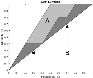
Figure 2.6:Example of a CAP Curve. Figure 2.7:Surfaces for AR.

[image:41.595.104.291.493.647.2]

(42)

power of the perfect model. Suppose A is the area between the perfect model curve and the random model curve (light plus dark gray area in 2.7), while B is the area between the rating model curve and random model curve (dark grey area in 2.7), then the AR is computed via Eq 2.17. For the example used the AR equals 44%.

AR = B

A + B (2.17)

Receiver Operating Characteristic

[image:42.595.150.481.337.476.2]

A concept that is closely related to the CAP curves is the Receiver Operating Character-istic (ROC). The ROC curve is constructed by using two distributions of rating scores for defaulting and non-defaulting debtors (BCBS, 2005).9 An example of possible distributions for rating scores can be found in Fig. 2.8.

Figure 2.8: Possible distributions for rating scores as found in BCBS (2005).

A perfect model would be able to separate the two distributions completely, but in practice it is more likely that they will overlap as is shown in Fig. 2.8 (BCBS, 2005). If you have to find out which debtors will default in the next period, it is possible to introduce a cut-off pointC, which results in the classification of potential defaulters (rating score belowC) and non-defaulters, who have a rating score above C (BCBS, 2005). High PD scores express the probability that a loan is likely to default, which typically if one uses credit risk scorecards result in low scores. Loans with a low probability to go into default usually have high scores. Thus, if only the PD values for each instance are available, the cut-off point represents a PD score. If an instance has a PD value above the cut-off point it will be classified as a default and if it has a lower PD value it will be classified as a non-default. The ROC is constructed by computing the Hit Rates (HR) and False Alarm Rates (FAR), via Eq. 2.18-2.19. TheHR

for eachCis the percentage that the model correctly classifies as default, whileFAR is the percentage of non-default that has been wrongly classified as default givenC.

HR(C) = H(C)

ND

(2.18)

9