Construction of energy savings cost curves: An application for Denmark

Munich Personal RePEc Archive

Construction of energy savings cost

curves: An application for Denmark

Pasquali, Andrea and Klinge Jacobsen, Henrik

Technical University of Denmark, DTU Management, Sustainability

Division

March 2019

Online at

https://mpra.ub.uni-muenchen.de/93076/

Construction of energy savings cost curves: An

application for Denmark

Andrea Pasquali & Henrik Klinge Jacobsen

Technical University of Denmark, DTU Management, Sustainability Division,

Produktionstorvet, 2800 Kgs Lyngby, Denmark, jhja@dtu.dk

Working Paper March 2019

ABSTRACT

This paper investigate the construction and use of energy saving cost curves. We discuss the various methodologies for calculating costs of savings measures and whether these can be compared across different sectors, end-uses and over time. The costs are fundamentally different if estimated as full cost of a measure, including installation, financing, transaction costs etc. or just the marginal cost of a more energy efficient component, for example type of glass or appliance model. We also highlight the difference in gross measures considered when examing option for residential building or industrial process equipment. Finally we introduce a few examples from Danish cost curves constructed and illustrate how different aggregation would be depending of which categories of costs are used in the construction of the corves.

INTRODUCTION

In the European Union, final energy use in the household and services sectors account for around 40 % of the overall consumption, whereas the industry roughly holds a 25 % share (Dalgleish et al., 2007; European Energy Agency, 2015). Figures at national level do not differ much from the EU trend. In Denmark, as reported by the Danish Energy Agency, households contributed to 31 % of the national final energy consumption in 2017 while industries and services to 33 % (Energistyrelsen, 2018). The same report expects the households share to fall down to 27 % in 2030, but foresees a 1.6 % annual rise in energy demand for industry and services in the same period (mainly due to an increasing diffusion of data centres). In the past years, building directives at national level as well as European guidelines have marked the need of reducing final end-use consumption (EU, 2010; Hansen & Hansen, 2015); institutions at all levels have strived for reaching energy and environmental targets that go in the direction of climate mitigation (Atanasui, 2011; Dalgleish et al., 2007; Erhorn & Erhorn-Kuttig Heike, 2015; European Parliament, 2009). This framework sets the grounds for large potential improvements in the efficiency of energy systems and technologies, and indirectly stresses the importance of designing appropriate policies to support them. Energy savings cost curves are broadly used tools to evaluate the cost-effectiveness of different investments and they are a key to rank and prioritize undertakings. Very often, they are utilized in combination with energy systems optimization models, e.g. to derive and define ad-hoc energy policies; in this case they are commonly referred to as aggregate cost curves. In some other situations, the private investor (for instance, in the form of a business) avails himself of savings cost curves to implement savings measures. Consequently, cost curves are employed to meet: on one hand the societal need of reducing energy consumption and greenhouse gas emissions; on the other, the private’s will to optimally reduce monetary expenditures for energy purposes.

Even if savings cost curves frequently appear when assessing industrial, commercial and residential investments, they generally fail to capture barriers, technological features and economical aspects that consistently affect the outcomes. In particular, they generally do not capture temporal dynamics, so that they can lead to a wrong estimation of saving potentials. This consideration is of utmost importance in the industrial world, where stock turnover and the replacement of obsolete, inefficient technologies constitute an essential step to stay competitive (Worrell, Ramesohl, & Boyd, 2004). In

short, assumptions regarding temporal parameters are of crucial relevancy for energy modellers and private investors and their influence is hardly considered in energy savings cost curves. The purpose of this paper is to analyze the way cost curves are usually built, highlighting flaws and suggesting possible refinements in their construction. The definition of a concerted method is crucial to allow for cross-sectoral and cross-national comparisons, so as to move from the interpretation of cost curves (Bühler, Guminski, et al., 2018) to a direct reading and usage.

EXPRESSING COSTS OF ENERGY SAVINGS MEASURES

The European Directive 2012/27/EU requires Member States to outline a strategy for encouraging renovation of the national building stock. The guidelines that function as a reference for the State’s action encompass the definition of tools that stimulate cost-effective renewal of buildings, and the implementation of policies that guide investments and decisions of individuals, the construction industry and stakeholders (Parliament, 2012). Cost curves are among these tools and help to visualize and properly evaluate the cost-effectiveness of investments. Several examples of the use of cost curves can be found in the literature, where they are applied to different, heterogeneous end-use sectors; however, the way they are built is not univocal, so that the lack of consistency hinders a comparison among diverse end-users and countries. More precisely, it is not often clear how costs are defined (Fleiter, Eichhammer, Wietschel, Hagemann, & Hirzel, 2009). One possible, common approach refers to implementation costs [EUR/kWh] (Bühler, Guminski, et al., 2018; Fleiter et al., 2009; Fleiter, Fehrenbach, Worrell, & Eichhammer, 2012; Zuberi & Patel, 2017), but it is often not explicit what these expenditures include: in particular, whether and energy savings are comprised or not in these calculations is not evident; (Toleikyte, Kranzl, & Müller, 2018) use also cost-effectiveness of investment, that is a levelized cost of energy expressed in terms of heated floor area [EUR/m2]. Other studies focus on the physical quantity that is being saved, not on energy itself (e.g. steam (Sathitbun-anan, Fungtammasan, Barz, Sajjakulnukit, & Pathumsawad, 2015) ). These last definitions are not suitable for comparisons among different sectors and political entities; expressing costs in terms of a saved physical quantity (e.g. steam) does not reveal much about energy savings potentials: for instance, steam value is not univocally determined. Furthermore, the concept of heated floor area is of wide use in the building sector, but a direct connection to energy savings lacks.

Some authors refer to Cost of Conserved Energy (CCE, [EUR/kWh]) as the quantity that better describes a saving potential (Fleiter et al., 2009; Hasanbeigi, Morrow, Sathaye, Masanet, & Xu, 2013; Mikulčić, Vujanović, & Duić, 2013; Morrow, Marano, Hasanbeigi, Masanet, & Sathaye, 2015; Toleikyte et al., 2018; Worrell, Martin, & Price, 2000). The advantages of using CCE instead of other financial methods are discussed in the literature (Martinaitis, Kazakevičius, & Vitkauskas, 2007). The principle behind this concept is to calculate the cost to save one energy unit and compare it to the energy price of that unit. From a normative point of view, the EU 244 2012 Directive specifies that global costs (which appear in the definition of CCE) need to be accounted for; they should include investment, running, energy and possibly disposal expenditures (EC 2012/C 115/01, 2012).Often, disposal costs are grouped together with the investment and technologies are assumed to hold no residual value (salvage) at the end of the lifetime. Running costs might be negative, as they can include earnings from produced energy. Various formal definitions for CCE have been proposed, adapted for different end-use sectors (Fleiter et al., 2009; Petersen & Svendsen, 2012); yet, they lack a substantial agreement on the inclusion of monetary savings. For this paper, the method described in (Fleiter et al., 2009) is considered and developed:

𝐶𝐶𝐶𝐶𝐶𝐶= 𝑎𝑎𝐼𝐼𝑚𝑚𝑚𝑚𝑚𝑚𝑚𝑚𝑚𝑚𝑚𝑚𝑚𝑚+𝑀𝑀𝑚𝑚𝑚𝑚𝑚𝑚𝑚𝑚𝑚𝑚𝑚𝑚𝑚𝑚− ∑ 𝛿𝛿·𝑝𝑝𝑗𝑗·𝐶𝐶𝑚𝑚𝑚𝑚𝑠𝑠𝑚𝑚𝑠𝑠,𝑗𝑗 𝑚𝑚

𝑗𝑗=1

∑𝑚𝑚𝑗𝑗=1𝛿𝛿·𝑓𝑓_𝑗𝑗·𝐶𝐶_{𝑚𝑚𝑚𝑚𝑠𝑠𝑚𝑚𝑠𝑠},𝑗𝑗 (1)

where a is the annuity factor for the investment obtained with the discount rate d, I represents the investment cost, M

the additional maintenance and running costs; 𝐶𝐶_{𝑚𝑚𝑚𝑚𝑠𝑠𝑚𝑚𝑠𝑠} is the amount of energy initially saved thanks to the implementation, corrected by a factor δ accounting for technology degradation and different economic lifetimes, should they vary among measures. The sum of annualized investment costs and maintenance expenditures are referred to as

global costs in the following. pj is the real retailprice of the energy commodity used for the normal functioning and fj is

the primary energy factor utilized to compare different qualities of energy. The summation is necessary when more than one energy carrier feeds the system (j represents an energy source). If only one is used, it is easy to see that investment and maintenance expenditures are corrected only by the factor 𝑝𝑝/𝑓𝑓, which contributes to value the saving investment. In addition, this suggests that investments requiring the same type of energy can be directly compared by considering investment and running costs, since −𝑝𝑝/𝑓𝑓 is a common constant. The formula adds value to measures which require carriers with low primary energy factors. Instead, and as a (relevant) example, let us assume a measure allows to save both electrical (1) and thermal (2) energy. This is often the case when one component is substituted in a rather complex system, where a device’s consumption is influenced by the other parts (e.g., a heat recovery unit in a ventilation system). The monetary savings per unit of conserved energy are (from (1)):

∑2𝑗𝑗=1𝛿𝛿·𝑝𝑝_𝑗𝑗·𝐶𝐶_{𝑚𝑚𝑚𝑚𝑠𝑠𝑚𝑚𝑠𝑠},𝑗𝑗

∑2𝑗𝑗=1𝛿𝛿·𝑓𝑓_𝑗𝑗·𝐶𝐶_{𝑚𝑚𝑚𝑚𝑠𝑠𝑚𝑚𝑠𝑠},𝑗𝑗 = 1

𝑓𝑓1

𝑝𝑝1 1 +𝐶𝐶2𝑓𝑓2

𝐶𝐶1𝑓𝑓1 +1

𝑓𝑓2

𝑝𝑝2 1 +𝐶𝐶1𝑓𝑓1

𝐶𝐶2𝑓𝑓2

= 𝑝𝑝1/𝑓𝑓1 1 +_{𝑒𝑒𝑓𝑓}1

+ 𝑝𝑝2/𝑓𝑓2

1 +𝑒𝑒𝑓𝑓 (2)

with e and f being respectively the ratio between different types of saved energy and the correspondent primary energy factors. Monetary savings still reduce the CCE, but taking into account also energy quality and the relative importance for the plant/service functioning (Figure 1). Due to the different quality of distinct energy carriers, it is necessary to weigh each energy saving with a primary energy factor (PEF). Such a consideration does not apply to monetary savings, since the different forms of energy are already weighted by their prices. pj is, in fact, the end-use price seen by the consumer.

Another discussion relate to the concept of net costs, where monetization of other benefits are deducted from the basic costs of the saving investment. That may be in the form of avoided externalities (Zvingilaite & Klinge Jacobsen, 2015) or additional comfort.

PRIMARY ENERGY FACTORS (PEF)

The practical evaluation of PEFs is the result of assumptions decided at national level, as the Building Directive approved by the European Parliament (The European Parliament and the Council of the European Union, 2010) delegates their assessment to Member States. Figures for the energy supply mix are, in fact, available at country level. Aside from unavoidable, physical discrepancies in the primary energy content of an energy carrier, the employed method (which is again a Member state’s choice) turns out to sharpen disomogeneity. As suggested in (Hitchin, Kingdom, Thomsen, & Wittchen, 2010), the EU should provide a clear and transparent method to calculate primary energy factors, so that local efforts and savings can be comparable through different states. In addition, Building Regulations generally don’t distinguish among different energy carriers, but set targets on the overall primary energy consumption of the building. Were cost curves built taking into account primary energy: a more direct relation with other Standards and directives would be achieved; a comparison between heating and electricity savings, thereby offering a direct perspective on which measures to prioritize for each end-use sector or category, would be both possible. In addition, the EU 244 2012 Directive recommends to assess costs (implementation, running, energy, disposal) at country level, regardless of geographical differences (EC 2012/C 115/01, 2012).

THE TEMPORAL DIMENSION

The approach embodied in Equation (2) works for measures that simultaneously influence the demand for manifold energy carriers, but can be utilized also for temporal considerations. As a matter of fact, issues related to the economic lifetime n are rarely addressed in cost curves. In general, it’s also unquestionable that a measure cannot be considered as effective as at the moment of the implementation for its entire lifetime. The following problems arise when dealing with the temporal dimension:

- Technological degradation (ξ). It is well-known that every energy efficiency measure is subject to degradation over time. The annual degradation (or deterioration) rate ξ strongly depends on the type of measure under consideration and it is linked to the maintenance effort (de Wilde, Tian, & Augenbroe, 2011). A savings cost curve is a ranking that shows how much energy can be saved on a yearly basis thanks to one (or a bundle of) undertaking(s), but this amount of energy is not constant over the lifetime. Literature on the topic is scarce, and rarely cost curves account for these inefficiencies. The result is an overestimation of the saving potential and a possible re-definition of the ranking. If including degradation rates in the construction of cost curves is not conceptually complicated, their determination is rather tricky. This is because of many factors, such as use, exposure, the interactions with other elements/devices (EC 2012/C 115/01, 2012), the presence of maintenance work. It is often hard to retrieve a reliable ξ even from manufacturers (Fleiter et al., 2009). However, considering the notable influence of degradation in the saving potential (de Wilde et al., 2011; Eleftheriadis & Hamdy, 2017; Waddicor et al., 2016), the error incurred in its estimation is generally more contained than when ξ is disregarded;

- Changes in the energy supply that require a re-definition of primary energy factors under use. As an example, a window is replaced. Currently, the building’s heating system includes an oil boiler for generation purposes, but in some years (within the lifetime of the measure) the dwelling will be connected to the district heating grid. The primary energy factor changes during the lifetime, but Equation (2) still holds true if weighting factors accounting for temporal variations are added. In alternative, the values can be averaged over the lifetime. For example, electrification of the heating sector represents a future tendency: as for Denmark, the Danish Energy Agency foresees an increase of 3.9 % in electricity consumption for heating purposes, on an annual basis. A similar jump is

expected for the industrial sector and household appliances (Energistyrelsen, 2018); therefore, PEFs undergo changes;

- Variations in the definition of primary energy factors at country level. The supply mix changes over time and primary energy factors are subject to a re-definition after a number of years, even if no change in technologies is undertaken by the end-user. The leanings towards higher shares of renewable energy in the generation mix and the improvements in energy conversion tend to reduce primary energy factors, whose estimates need accuracy (and possibly uniformity).

- Trend and volatility of a commodity’s price. This constitutes one of the biggest sources of uncertainty in cost assessment (Hassett & Metcalf, 1993). Future prices of the most common energy carriers are suggested in (EC 2012/C 115/01, 2012) and can serve as a possible benchmark for modelling purposes.

- Time required for the measure implementation. Radical changes in the building envelope or certain replacements may call for long transition periods.

As a matter of fact, the measures included in the same cost curve have dissimilar expected lifetimes, and that should be taken into account as well when prioritizing cost-effective undertakings. For this reason, the constant

𝛿𝛿=𝑘𝑘𝑓𝑓(𝜉𝜉)

incorporated in Equation (1), includes k, that penalizes measures with shorter lifetimes. k is calculated as the ratio of the the lifetime of the considered measure and the biggest lifetime in the curve. This reasoning is pertinent as long as the overall objective is simply a reduction of final energy consumption. The coefficient accounting for technological degradation, 𝑓𝑓(𝜉𝜉), is computed as an integral mean, over the measure’s lifetime n (it is assumed that at year 1 the measure has full efficiency):

𝑓𝑓(_𝜉𝜉) = (1− 𝜉𝜉) 𝑛𝑛−1₋₁

ln(1− 𝜉𝜉) (𝑛𝑛 −1) (3)

These rather simple calculations allow to make up for substantial mistakes in the assessment of the saving potential. Equation (3) shows that this misevaluation grows bigger with high ξ and long lifetimes n. In short, an assessment of the saving potentials should account for: their duration; the inherent drop in the effectiveness of the measure; external (relevant) changes that influence the supply mix and the energy price throughout the expected lifetime.

TEMPORAL DIMENSION: AN EXAMPLE

An illustrative example accouting for different economic lifetimes and degradation rates is provided in Table 1. The two measures are supposed to reduce the consumption of one definite energy carrier.

Table 1. Influence of lifetime and degradation rate on the CCE.

I M Esaved d Lifetime ξ δ p f CCE

(old) CCE (new) Measure 1 5000 100 1000 4 20 1 0.913 0.1 1 0.368 0.412

Measure 2 5000 100 1500 4 15 1.2 0.692 0.1 1 0.267 0.430

A separate issue is the value of energy savings as different hourly profiles for energy savings, especially electricity can influence the net costs of energy savings substantially as for example investigated by (Klinge Jacobsen & Juul, 2015).

DISCOUNT RATES

Discount rates give a present value to future expenditures and earnings (EU, 2014) and they are among of the most influential parameters in the evaluation of CCE. As explicitly stated in (EC 2012/C 115/01, 2012), a sensitivity analysis on discount rates is necessary to evaluate the impact on financial calculations. It is common practice to distinguish between social and private discount rates, as they represent diverse investors and therefore needs and expectations. Social discount rates are generally smaller than private discount rates (Bruderer Enzler, Diekmann, & Meyer, 2014; García-Gusano, Espegren, Lind, & Kirkengen, 2016; Hassett & Metcalf, 1993; Hoffman et al., 2015; Newell & Siikamki, 2015); this follows as a consequence of several factors, but it mainly reflects the more risky nature of private investments, the presence of market imperfections (García-Gusano et al., 2016) and the time horizon for the investment to generate utility (Bruderer Enzler et al., 2014). That is to say, a private investor generally desires to be repaid of the investment in a shorter amount of time; society instead tends to plan for the long-term. Nevertheless, there is not a complete agreement on the factors that justify the adoption of different figures for social and private (or financial (EU, 2014)) discount rates (Worrell et al., 2004). Indeed, both represent an opportunity-cost of capital, but the first embraces an inter-temporal, cross-generational perspective. The determination of discount rates is rather intricate because of the amount of intertwined parameters that contribute to their calculation; ultimately, not only a single figure is asked to encapsulate several qualitative inputs, but also to synthesize behavioural aspects, market and cultural barriers (Worrell et al., 2004). In case a discount rate is to be applied, it should be considered that also socio-economic determinants are decisive in differentiating across investors: income, education, gender, age are among these parameters. For these reasons, the investor’s perspective cannot be fully described by the only use of the market price of capital; it should also depend on an individual’s characteristics, risk assessment and expectations about the future (Steinbach & Staniaszek, 2015). In most

Figure 1. Cost of conserved energy accounts for implementation costs and energy savings.

Sp

e

ci

fi

c

sa

vi

n

gs

|

Sp

e

ci

fi

c

co

st

s

[

E

U

R/k

W

h

]

Saving potential [kWh]

Cost term

Monetary savings

Cost of Conserved Energy

cases, the undeniable subjectivity that this time-demanding synthesis requires forces investors and modellers to neglect a large part of these contributions, thereby increasing the probability of an improper discounting. The context where the investment takes place is also of relevance in determining the discount rate. Industrial replacements and refurbishments are expected to quickly pay off, as business dynamics call for frequent modernization to hold competitiveness: therefore, industrial and commercial investors should be modelled with a higher discount rate than small investors (households). In general, energy savings measures are illiquid and perceived as irreversible (Sutherland, 1991), so that the desired rate of return is high. The choice of the discount rate also markedly influences the effect of future costs. In other words, as the discount rate increases, future costs weigh less on the CCE (García-Gusano et al., 2016). This consideration gains more importance when OPEX are consistent, i.e. often in the case of active measures.

In short, the adoption of a certain discount rate carries along a series of uncertainties and forces to build on rather strong assumptions; there exist manifold categories of investors and contexts that complicate cross-comparisons among different sectors.

COSTS CALCULATION

When applying Equation (1), two approaches are possible as far as costs calculations are concerned(Fleiter et al., 2009; Zuberi & Patel, 2017):

- one considers full costs, which consist of all the expenditures related to the measure implementation (including installation). A comparison is carried out between the new, potential situation and the current state and characteristics of the components;

- another utilizes additional (marginal) costs, i.e. the comparative advantage of investing in a certain energy-efficient measure with respect to a standard technology that serves the same purpose (two windows with different U-values, two heat recovery systems with diverse efficiencies etc.). In this case, I and M in Equation (1) are to be thought as delta values instead.

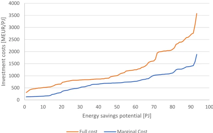
In other words, full costs do not imply that people invest in any event, but make use of ex-ante consumption. The two methods may lead to considerably different results, especially in countries where the labor cost is high (Zuberi & Patel, 2017), and are in general highly dependent on the measure; besides, the approaches can prioritize different undertakings. The adoption of either full or marginal costs might depend on several circumstances (Figure 2 explains how full and marginal costs relate with each other and with the saving potential.

When a measure is implemented, a series of side effects follow. They are generally hard to quantify and monetize. Some concern energy consumption, the most relevant being the rebound effect. Others are linked benefits that appear either in other components, elements, assets or that influence the human perception of the environment. Examples are increased productivity and product quality, noise reduction, add on property value and indirect financing to other renovation projects. These factors are rarely accounted for also to lighten the creation of cost curves, but may be kept in mind especially in the case of private investments.

TYPE OF MEASURE

The definition of global costs in the EU Directive 244 2012 reinforces the distinction between active and passive measures. Even if not systematic, this differentiation is present in the literature (Units, Depict, Model, & Athens, 2016). Passive measures aim at improving the building envelope and are characterized by null energy consumption during their

Figure 2. Visual comparison between full and marginal costs.

lifetime; on the contrary, active measures concern appliances, plants, equipment1 and their operation: therefore, they require energy to run. This distinction is convenient because interventions that belong to the same category have rather homogenous attributes, such as technical reliability, degradation rates or persistence (Hoffman et al., 2015) and economic discounting (Hansen & Hansen, 2015). These features are often object of sensitivity analyses to evaluate their impact under different assumptions. As an example, in the Danish Building Regulation 15 (Hansen & Hansen, 2015), building elements, windows, ventilation ducts and heating systems have an expected technical lifetime of 30-40 years, whereas heat appliances, lighting, building automation are supposed to last for 15-20 years. In an industrial context, plants have generally a shorter lifetime and are exposed to high renovation rates; some authors suggest that architectural and constructive components have a life-cycle time that is at least threefold the one of a plant (Units et al., 2016). In short, an active measure:

- carries along additional categories of costs (or benefits). Its OPEX are a relevant part of the global costs and need to be accounted for in the decision-making process; in particular, variations in energy prices may influence the global costs;

- has a shorter lifetime. Besides, its technical lifetime (which is usually considered and reported in official documents) may considerably differ from its economic lifetime, i.e. the amount of time a service is profitable rather than usable. When evaluating the implementation costs of a measure, these factors are relevant;

- may be characterized by different discount rates than the ones of a passive measure.

As a consequence, this classification establishes another criterion for undertaking the investment: active measures are generally prioritized when a ranking is created. However, this approach: may lead to an oversizing of the plant/services, if further structural ameliorments are considered afterwards; neglects the fact that several studies suggest to act on the building envelope to enhance cost-effectiveness (Units et al., 2016). In short, other aspects can condition the choice of one or the other measure: these are typically related to the prioritization of monetary over energy savings. They are often the results of bounded rationality and they are generally difficult to render; therefore, they are neglected in the construction of cost curves.

UNCERTAINTY

All the assumptions establish a certain degree of uncertainty, this being a relevant influence when building and critically assessing savings cost curves. The effect is accentuated in the case of active measures. Uncertainty is seldom addressed in the literature, even though an attempt can be found in (Bühler, Petrović, et al., 2018); the degree to which defined parameters condition energy savings ranges in an interval whose breadth hangs on the specific end-use sector. In (Golove & Eto, 1996), it is underlined how the private investor can aim at diversifying risk above all, thereby moving away from the energy savings effort. When applying Equation (1) in an industrial context, fluctuation in the short- or long-term production as well as in other external, meaningful decision variables (e.g. weather) enlarge the uncertainty of energy savings estimates: in (Bühler, Petrović, et al., 2018), the authors address this issue with the aid of Monte Carlo simulations, both for the saving potential and the cost of implementation; in (Kelly Kissock & Eger, 2008), it is acknowledged that energy savings estimates may differ from actual measurements, but the authors rely on ex-post metering for a post-implementation assessment, which lies outside the predictive potential of cost curves. These considerations apply only for the cost term in (1). In fact, in the case of active measures, the amount of energy saved can be rewritten as the power consumed by the measure, for each specific energy source, 𝑃𝑃_𝑗𝑗 and the component’s full load hours flh:

𝐶𝐶𝐶𝐶𝐶𝐶𝑓𝑓=𝑎𝑎𝐼𝐼

+𝑀𝑀 − ∑𝑚𝑚𝑗𝑗=1𝑝𝑝_𝑗𝑗·𝐶𝐶_{𝑚𝑚𝑚𝑚𝑠𝑠𝑚𝑚𝑠𝑠},𝑗𝑗

∑𝑚𝑚𝑗𝑗=1𝑓𝑓𝑗𝑗·𝐶𝐶𝑚𝑚𝑚𝑚𝑠𝑠𝑚𝑚𝑠𝑠,𝑗𝑗

= 𝑎𝑎𝐼𝐼+𝑀𝑀

𝑓𝑓𝑓𝑓ℎ ∑𝑚𝑚𝑗𝑗=1𝑓𝑓𝑗𝑗·𝑃𝑃𝑗𝑗−

∑𝑚𝑚𝑗𝑗=1𝑝𝑝𝑗𝑗·𝑃𝑃𝑗𝑗

∑𝑚𝑚𝑗𝑗=1𝑓𝑓𝑗𝑗·𝑃𝑃𝑗𝑗

(3)

The uncertainty (due e.g. to production, weather, …) in the full-cost approach 𝐶𝐶𝐶𝐶𝐶𝐶_𝑓𝑓 is taken on by the cost term only; full load hours represent the operations of the plant (appliance, service etc.) and they are independent on the various energy carriers. If marginal cost curves are built, delta values should be considered instead. The derivative of (3) with respect to

flh is negative in its entire domain and its mathematical expression is in the form of −𝑐𝑐/𝑓𝑓𝑓𝑓ℎ2, with c positive constant. As a consequence: plants (appliances, services) that are run for little time during the year are more sensitive to uncertainty;

1

Equipment can be included into this category, however from a regulatory point of view, energy consumption focuses on heating, DHW, ventilation, cooling, lighting. Equipment is not really considered.

the chosen approach, i.e. full or marginal costs, by influencing the constant k, impacts on the size of deviation from the forecasted and the actual CCE (which is a function of full load hours).

THE RELATIONSHIP WITH REGULATIONS

Building Regulations (at national level) require new and old buildings subject to renovation to fulfill precise requirements in terms of primary energy consumption (Hansen & Hansen, 2015). Certainly, in recent years a rather large debate on the concepts of renovation, retrofit, refurbishment has produced a series of papers and documents that aim at defining each of the previous as well as at harmonising different sensibilities; notwithstanding, these terms are often confused and employed as if they were interchangeable. As thoroughly illustrated in (Deep & Definition, 2013), renovation implies the most drastic changes, mainly (but not only) concerning the building envelope; retrofitting rather singles out interventions on the mechanical systems. Some effort has also been put in determining quantitatively which targets are to be attained in case of ‘deep renovation’. According to (GBPN, What is a deep renovation), deep renovation occurs when primary energy consumption is reduced by at least 75 % compared to the status quo; moreover, the overall primary energy consumption for heating, cooling, lighting, ventilation and domestic hot water should not exceed a threshold of 60 kWh/m2/year. In other words, deep renovation requires intervention by means of both active and passive measures. What this classification includes reflects mainly the European sensibility. In the US, such an absolute target would encompass all possible sources of consumption, thereby comprising appliances (Deep & Definition, 2013). It is relevant to point out that the current Danish Building Regulation (Hansen & Hansen, 2015) forces old (but under renovation) dwellings to comply with different, weaker requirements. In the document, two classes of renovated dwellings are considered. Table 2 provides a picture of these conditions.

Table 2. Primary energy requirements for buildings under renovation. A [m2] stands for the heated floor area.

Renovation class 1 [kWh/m2/year]

Renovation class 2 [kWh/m2/year] Dwellings, student accommodations,

hotels

52.5 + 1650/A 110 + 3200/A

Offices, schools, institutions 71.3 + 1650/A 135 + 3200/A

In Denmark, requirements are still expressed in function of the building heated floor area A, therefore a direct comparison with an absolute threshold is impossible (maybe include statistics on national average floor area?) It seems legit to refer to Renovation class 1 as ‘deep renovation’. ‘Standard renovation’ (or ‘shallow renovation’) instead can be referred to as Renovation class 2. The previously mentioned (Deep & Definition, 2013) defines as ‘Standard renovation’ an intervention that results in savings ranging from 20 to 30 % with respect to the initial consumption. A comparison with Denmark is here impossible, since only a relative target is defined.

According to the same source, ‘deep retrofit’ is achieved with a 50 % reduction and, as previously mentioned, is mainly related to the replacement of systems and plants. These guidelines are primarily valid for the existing building stock, whereas literature on the topic is lacking for industry. The Danish Building Regulation does not distinguish between retrofit and renovation. Little harmonisation among directives and regulations does not help to clearly determine how deep renovation is attained; the EU’s Energy Performance of Buildings Directive suggests Member States to define ‘major renovation’ in terms of either the value of the building or a percentage of the building envelope subject to the intervention (EU, 2010). Regardless of specific figures and of the directive chosen as a reference, several studies recommend to prefer strong over weak renovation measures, the qualitative discrepancy between the two being the combined intervention on systems, plants and building envelope when the former is undertaken (Semprini, Gulli, & Ferrante, 2017). This outcome is justified by economic analyses that, with the use of Net Present Value (NPV), show how a financial return on investment is rarely achieved with a superficial intervention (for instance, (Semprini et al., 2017)). Furthermore, the cost-effectiveness of policies promoting shallow renovation with a strong share of renewables in the supply mix was proved to be inferior to a scenario with strong energy efficiency measures (“Deep renovation of buildings An effective way to decrease Europe ’ s energy import dependency Deep renovation of buildings An effective way to decrease Europe ’ s energy import dependency,” n.d.) Without doubts, the concept of deep renovation implies a substantial change in the nature of the building, the factory and the systems present therein. The confusion arising from poorly harmonized directives and mismatching definitions makes the identification of quantitative energy savings targets more complicated. This is concretely due to:

- confusion in the use of terms, which are often treated as completely interchangable;

- the definition of both relative and absolute targets. Relative targets are associated with ex-ante energy consumption, which often do not match the demand, i.e. the energy a building is foreseen to consume at the design

stage. This is assessed with the use of simulation environments, that is, not accounting for design flaws, behavioural aspects and other unpredictable events.

Even if the utlimate goal is clear, how this is to be reached is not. For comparison purposes, the lack of an agreement on definitions and targets makes efforts complicated when not impossible.

0 500 1000 1500 2000 2500 3000 3500 4000

0 10 20 30 40 50 60 70 80 90 100

In

ve

st

m

e

n

t

co

st

s [M

E

U

R

/P

J]

Energy savings potential [PJ]

Full cost Marginal Cost

Figure 3. Example from DK difference between marginal and full costs

References

Atanasui, B. (2011). FinAl drAFt PrinciPles For neArly Zero-energy Buildings. Buildings. Retrieved from http://www.bpie.eu/nearly_zero.html

Bruderer Enzler, H., Diekmann, A., & Meyer, R. (2014). Subjective discount rates in the general population and their predictive power for energy saving behavior. Energy Policy, 65, 524–540. https://doi.org/10.1016/j.enpol.2013.10.049

Bühler, F., Guminski, A., Gruber, A., Nguyen, T. Van, von Roon, S., & Elmegaard, B. (2018). Evaluation of energy saving potentials, costs and uncertainties in the chemical industry in Germany. Applied Energy, 228(December 2017), 2037–2049.

https://doi.org/10.1016/j.apenergy.2018.07.045

Bühler, F., Petrović, S., Ommen, T., Holm, F. M., Pieper, H., & Elmegaard, B. (2018). Identification and Evaluation of Cases for Excess Heat Utilisation using GIS. Energies, 1–24. https://doi.org/10.3390/en11040762

Dalgleish, T., Williams, J. M. G. ., Golden, A.-M. J., Perkins, N., Barrett, L. F., Barnard, P. J., … Watkins, E. (2007). [ No Title ]. Journal of Experimental Psychology: General, 136(1), 23–42.

de Wilde, P., Tian, W., & Augenbroe, G. (2011). Longitudinal prediction of the operational energy use of buildings. Building and Environment, 46(8), 1670–1680. https://doi.org/10.1016/j.buildenv.2011.02.006

Deep renovation of buildings An effective way to decrease Europe ’ s energy import dependency Deep renovation of buildings An effective way to decrease Europe ’ s energy import dependency. (n.d.).

Deep, W. I. S. a, & Definition, R. (2013). What Is a Deep, (February), 237–254.

EC 2012/C 115/01. (2012). Commission Delegated Regulation (EU) No 244/2012 of 16 January 2012 supplementing Directive 2010/31/EU of the European Parliament and of the Council on the energy performance of buildings by establishing a comparative methodology framework for calculating. Official Journal of the European Union, 28. https://doi.org/10.3000/1977091X.C_2012.115.eng

Eleftheriadis, G., & Hamdy, M. (2017). Impact of building envelope and mechanical component degradation on the whole building performance: A review paper. Energy Procedia, 132, 321–326. https://doi.org/10.1016/j.egypro.2017.09.739

Energistyrelsen. (2018). Denmark’s Energy and Climate Outlook 2018 Baseline Scenario Projection Towards 2030 With Existing Measures (Frozen Policy) Denmark’s Energy and Climate Outlook 2018: Baseline Scenario Projection Towards 2030 With Existing Measures (Frozen Policy). Retrieved from http://www.ens.dk

Erhorn, H., & Erhorn-Kuttig Heike. (2015). Nearly Zero- Energy Buildings, (April). Retrieved from http://www.epbd-ca.eu/outcomes/2011-2015/CA3-CT-2015-5-Towards-2020-NZEB-web.pdf

EU. (2010). Directive 2010/31/EU of the European Parliament and of the Council of 19 May 2010 on the energy performance of buildings (recast).

Official Journal of the European Union, 13–35. https://doi.org/doi:10.3000/17252555.L_2010.153.eng

EU. (2014). Guide to Cost-benefit Analysis of Investment Projects: Economic appraisal tool for Cohesion Policy 2014-2020. Publications Office of the European Union. https://doi.org/10.2776/97516

European Energy Agency. (2015). Final energy consumption by sector and fuel. Indicator Assessment | Data and Maps, 20. https://doi.org/CSI 027/ENER 016

European Parliament. (2009). "Decision No 406/2009/EC of the European Parliament and of the Council ". Official Journal of the European Union,

L140, 136–148. https://doi.org/10.2779/57220

Fleiter, T., Eichhammer, W., Wietschel, M., Hagemann, M., & Hirzel, S. (2009). Costs and potentials of energy savings in European industry - a critical assessment of the concept of conservation supply curves. Proceeding ECEEE 2009, (May 2014), 1261–1272. Retrieved from

https://www.etde.org/etdeweb/details_open.jsp?osti_id=967850

Fleiter, T., Fehrenbach, D., Worrell, E., & Eichhammer, W. (2012). Energy efficiency in the German pulp and paper industry - A model-based assessment of saving potentials. Energy, 40(1), 84–99. https://doi.org/10.1016/j.energy.2012.02.025

García-Gusano, D., Espegren, K., Lind, A., & Kirkengen, M. (2016). The role of the discount rates in energy systems optimisation models. Renewable and Sustainable Energy Reviews. https://doi.org/10.1016/j.rser.2015.12.359

Golove, W. H., & Eto, J. H. (1996). Market Barriers to Energy Efficiency : A Critical Reappraisal of the Rationale for Public Policies to Promote Energy Efficiency. Energy Environment, 26(March), 66. https://doi.org/10.1177/0042098011427189

Hansen, C. F., & Hansen, M. L. (2015). Executive Order on the Publication of the Danish Building Regulations 2015 (BR15), 2015(1185). Hasanbeigi, A., Morrow, W., Sathaye, J., Masanet, E., & Xu, T. (2013). A bottom-up model to estimate the energy efficiency improvement and

CO2emission reduction potentials in the Chinese iron and steel industry. Energy, 50(1), 315–325. https://doi.org/10.1016/j.energy.2012.10.062

Hassett, K. A., & Metcalf, G. E. (1993). Energy conservation investment. Do consumers discount the future correctly? Energy Policy, 21(6), 710–716. https://doi.org/10.1016/0301-4215(93)90294-P

Hitchin, R., Kingdom, U., Thomsen, K. E., & Wittchen, K. B. (2010). Primary Energy Factors and Members States Energy Regulations, (692447).

Hoffman, I. M., Schiller, S. R., Todd, A., Billingsley, M. A., Goldman, C. A., & Schwartz, L. C. (2015). Energy Savings Lifetimes and Persistence: Practices, Issues and Data. Technical Brief – Electricity Markets & Policy Group. Berkeley, California, United States.

Kelly Kissock, J., & Eger, C. (2008). Measuring industrial energy savings. Applied Energy, 85(5), 347–361. https://doi.org/10.1016/j.apenergy.2007.06.020

Klinge Jacobsen, H., & Juul, N. (2015). Demand-side management: electricity savings in Danish households reduce load variation, capacity

requirements, and associated emissions @ DTU International Energy Report 2015 : Energy systems integration for the transition to non-fossil energy systems.

Martinaitis, V., Kazakevičius, E., & Vitkauskas, A. (2007). A two-factor method for appraising building renovation and energy efficiency improvement projects. Energy Policy, 35(1), 192–201. https://doi.org/10.1016/j.enpol.2005.11.003

Mikulčić, H., Vujanović, M., & Duić, N. (2013). Reducing the CO2 emissions in Croatian cement industry. Applied Energy, 101, 41–48. https://doi.org/10.1016/j.apenergy.2012.02.083

Morrow, W. R., Marano, J., Hasanbeigi, A., Masanet, E., & Sathaye, J. (2015). Efficiency improvement and CO2emission reduction potentials in the United States petroleum refining industry. Energy, 93, 95–105. https://doi.org/10.1016/j.energy.2015.08.097

Newell, R. G., & Siikamki, J. (2015). Individual time preferences and energy efficiency. In American Economic Review (Vol. 105, pp. 196–200). https://doi.org/10.1257/aer.p20151010

Parliament, E. (2012). L 81/18, 18–36.

Petersen, S., & Svendsen, S. (2012). Method for component-based economical optimisation for use in design of new low-energy buildings.

Renewable Energy, 38(1), 173–180. https://doi.org/10.1016/j.renene.2011.07.019

Sathitbun-anan, S., Fungtammasan, B., Barz, M., Sajjakulnukit, B., & Pathumsawad, S. (2015). An analysis of the cost-effectiveness of energy efficiency measures and factors affecting their implementation: a case study of Thai sugar industry. Energy Efficiency, 8(1), 141–153. https://doi.org/10.1007/s12053-014-9281-7

Semprini, G., Gulli, R., & Ferrante, A. (2017). Deep regeneration vs shallow renovation to achieve nearly Zero Energy in existing buildings: Energy saving and economic impact of design solutions in the housing stock of Bologna. Energy and Buildings, 156, 327–342.

https://doi.org/10.1016/j.enbuild.2017.09.044

Steinbach, J., & Staniaszek, D. (2015). Discount rates in energy system analysis. Buildings Performance Institue Europe (BPIE), (May). Sutherland, R. J. (1991). Market barriers to energy-efficiency investments. Energy Journal, 12(3), 15. Retrieved from

http://search.ebscohost.com/login.aspx?direct=true&db=afh&AN=9610284496&site=ehost-live

The European Parliament and the Council of the European Union. (2010). Directive 2010/30/EU on the indication by labelling and standard product information of the consumption of energy and other resources by energy-related products. Official Journal of the European Union, (4), 1–12. https://doi.org/10.1017/CBO9781107415324.004

Toleikyte, A., Kranzl, L., & Müller, A. (2018). Cost curves of energy efficiency investments in buildings – Methodologies and a case study of Lithuania.

Energy Policy, 115(December 2017), 148–157. https://doi.org/10.1016/j.enpol.2017.12.043

Units, U., Depict, T. O., Model, A. C., & Athens, F. O. R. (2016). Nearly Zero Energy Urban Settings ( ZEUS ). https://doi.org/10.1016/B978-0-08-100735-8/00002-7

Waddicor, D. A., Fuentes, E., Sisó, L., Salom, J., Favre, B., Jiménez, C., & Azar, M. (2016). Climate change and building ageing impact on building energy performance and mitigation measures application: A case study in Turin, northern Italy. Building and Environment, 102, 13–25. https://doi.org/10.1016/j.buildenv.2016.03.003

Worrell, E., Martin, N., & Price, L. (2000). Potentials for energy efficiency improvement in the US cement industry. Energy, 25(12), 1189–1214. https://doi.org/10.1016/S0360-5442(00)00042-6

Worrell, E., Ramesohl, S., & Boyd, G. (2004). Advances in Energy Forecasting Models Based on Engineering Economics. Annual Review of Environment and Resources, 29(1), 345–381. https://doi.org/10.1146/annurev.energy.29.062403.102042

Zuberi, M. J. S., & Patel, M. K. (2017). Bottom-up analysis of energy efficiency improvement and CO2emission reduction potentials in the Swiss cement industry. Journal of Cleaner Production, 142, 4294–4309. https://doi.org/10.1016/j.jclepro.2016.11.178

Zvingilaite, E., & Klinge Jacobsen, H. (2015). Heat savings and heat generation technologies: Modelling of residential investment behaviour with local health costs. Energy Policy, 77, 31–45. https://doi.org/10.1016/j.enpol.2014.11.032