Estimating threshold level of inflation in Swaziland: inflation and growth

(1)

Munich Personal RePEc Archive

Estimating threshold level of inflation in

Swaziland: inflation and growth

Mosikari, Teboho Jeremiah and Eita, Joel Hinaunye

North-West University, South Africa, University of Johannesburg

25 January 2018

(2)

1

Estimating threshold level of inflation in Swaziland: inflation and growth

Teboho Jeremiah Mosikari

School of Economic and Management Science Department of Economics

North West University South Africa

E-mail: tebohomosikari@gmail.com

Joel Hinaunye Eita

School of Economics, College of Business and Economics

University of Johannesburg South Africa

E-mail: jeita@uj.ac.za or hinaeita@yahoo.co.uk

Abstract

The objective of this study is to estimate optimal threshold effect of inflation for the economy of Swaziland. The study applied the liner OLS and Two-Stage least squares (2SLS) methods to determine the optimal effect of inflation on growth. It used annual data for the period 1980 to 2015. The results of liner OLS method show that the estimated optimal threshold level is at 12%. The results show that inflation rate beyond optimal level of 12% decrease growth by 1.02%. Similar results were also found in applying 2SLS method, where inflation exerted a negative impact beyond threshold point by 18.5%. These findings on Swaziland economy have crucial implications for monetary policy makers in terms of keeping inflation below the threshold point to sustain a positive economic growth in the long run.

JEL classification: B22, C01, E31, O40

(3)

2

1. Introduction

The interest of each economic policy maker is to sustain high economic growth with stable

price levels. Inevitably, it is well known that policy makers are expected to make tradeoff in

maintain policies that combat inflation without harming potential economic growth. Hasanov

(2011) explained that to maintain suitable economic growth and price levels simultaneously,

can be hard to accomplish for economic policy makers. Although there is a vast debate about

the negative effect of inflation on output growth, however there appears to be a consensus

among economists that macroeconomic stability, specifically defined as low inflation, is

negatively related to economic growth (Sindano, 2014). According to Bawa and Abdullahi

(2012) severe inflation has several consequences such that firstly, it impose welfare cost to the

society. Secondly, it discourage savings and investment by creating uncertainty about the future

prices. Thirdly, it cost the low income households by reducing their purchasing power. Finally,

it minimise the country‘s exports competitiveness due to relative prices and negatively impact

on the trade account.

Literature clearly indicates some frameworks concerning the relationship between inflation and

economic growth. The study by Seleteng (2005) highlighted some theories such as Keynesian

theory and monetarism which can be used to predict the expected relationship between inflation

and economic growth. The Keynesian theory suggest that there is positive relationship between

inflation and output in the long run. This could be due to some firms may agree to supply some

goods at the later stage. The other possibility is that during full employment in aggregate

demand (AD) and aggregate supply (AS) model, continuous increase in AD will lead to

inflationary state. The theory on monetarism suggest that in the long run prices are affected by

an excessive supply of money. This notion of theory was pioneered by Friedman (1956) in his

(4)

3 economic growth suggests that there is a possible positive association among the variables. An

analysis on the relationship between inflation and economic growth in Swaziland is of

paramount importance. Like many developing economies, Swaziland citizens are faced with

higher prices in their everyday life. Figure 1 depicts the relationship between inflation and

economic growth in Swaziland for the period 1980 to 2015. Inflation rate trended in double

digits and was detrimental to economic growth during the period 1980 to 1990. During the

period 1990 to 2004 inflation rate grew above economic growth with approximately an average

growth rate of 6% per year. During the periods, respectively 1988 and 1990, Swaziland’s

economic growth rate was above 6%. This was the highest growth experiences in Swaziland.

The economy of Swaziland witnessed low economic growth during 2010 and 2011, and this

was due to the aftermath of the financial crisis (UNECA1_{, 2016). It can be concluded from the}

figure that there is positive relationship between inflation and economic growth for the period

[image:4.595.76.546.456.705.2]

1980 to 2015.

Figure 1: Swaziland’s inflation rate and real GDP growth rate for the period 1980 to 2015

Source: Own compilation using data from IMF

1_{United Nations Economic Commission for Africa} -10.00

-5.00 0.00 5.00 10.00 15.00 20.00 25.00

1980 1981 1982 1983 1984 1985 1986 1987 1988 1989 1990 1991 1992 1993 1994 1995 1996 1997 1998 1999 2000 2001 2002 2003 2004 2005 2006 2007 2008 2009 2010 2011 2012 2013 2014 2015

p

e

rce

n

ta

ge

ch

an

ge

(5)

4 In a small developing economy like Swaziland, unstable price levels have a prospective

detrimental effect on economic growth in the long run. Extensive empirical studies on

determining the optimal threshold point of inflation in Swaziland are scarce, and limited to one

study by Mkhatshwa, Tijani and Masuku (2015). The study indicates that there is a long run

relationship between inflation and economic growth in Swaziland. The study used non-liner

OLS to estimate 12% optimal threshold level of inflation that discouraging economic growth

in Swaziland. In the essence of the role and the importance of inflation in an economy, it is

imperative to investigate the threshold point of inflation on economic growth. The main

purpose of this study is to examine whether there is any optimal threshold effect of inflation

on economic growth in Swaziland. This study contributes to the literature firstly by using

different control variables following the ones used and explored Mubarik (2005), Seleteng

(2005) and Khan and Senhadji (2001). Lastly, unlike the study of Mkhatshwa, Tijani and

Masuku (2015) that used non-linear method, the current study uses linear approach by applying

basic OLS and Two-Stage Least Squares (2SLS). The rest of this study is organised as follows.

Section 2 presents empirical literature on inflation and economic growth. Section 3 provides

model specification. Section 4 discusses methodology and data. Section 5 reports estimation

results. Lastly, Section 6 conclude the study.

2. Empirical literature

There is a large literature investigatingempirical andtheoretical relationship between inflation

and output growth. However, this vast literature consists of two types of studies that investigate

the relationship between inflation and economic growth. One set of studies specifically

concentrate on the relationship between inflation and output growth. This kind of studies

(6)

5 growth. Another set of studies argue that there an optimal level where inflation may be harmful

to output growth. This current study will focus on studies that investigated the optimal level of

inflation on economic growth. Vinayagathasan (2013) studied inflation and growth for 32

Asian countries. The study used panel dynamic threshold model for the period 1980 to 2009.

The study found that inflation hurts economic growth when it exceeds 5.43%. The results also

indicated that inflation rate below 5.43% did not have any effect on growth. Alkahtani and

Elhendy (2014) examined the optimal level of inflation rate in the Kingdom of Saudi Arabia.

The study found that the optimal level of inflation that is harmful for economic growth in Saudi

Arabia ranged from 3% to 4%.

Yabu and Kessy (2015) investigated threshold level of inflation for economic growth of three

founding East African Community (EAC) member states. These member states are Kenya,

Tanzania and Uganda. The paper applied panel analysis methods such as random effects (RE)

andseemingly unrelated regression (SUR) for the period1970 to 2013. The results indicate

that the average rate of inflation beyond 8.46% is harmful to economic growth. Recent

empirical study by Bhusal and Silpakar (2011) explored the nexus between inflation and

economic growth and to determine the threshold level of inflation for Nepal. The results of the

study show that the threshold value of inflation is found to be 6% for Nepal. Bawa and

Abdullahi (2012) studied an optimal threshold effect of inflation on economic growth in

Nigeria. The results shown a threshold inflation level of 13% for Nigeria, which implies that

below this level, inflation has insignificant impact on economic growth.

There is a general consensus that policy makers and central bankers acknowledge that the main

(7)

6 a low inflation rate. Rutayisire (2013) investigated the relationship between inflation and

growth in the economy of Rwanda for the period spanning from 1968 to 2010. The study used

the quadratic model to determine whether there is a turning point level of inflation, at which

the inflation starts to negatively impact on output growth. Rutayisire (2013) found out that

estimated inflation threshold level is 14.97%. Inflation rate of above 14.97% is detrimental to

output growth of Rwanda. Makuria (2013) studied the relationship between inflation and

economic growth in Ethiopia. The study used a quarterly dataset from 1992Q1 to 2010Q4. The

study applied Engle-Granger and Johansen co-integration tests and determine if there is a

long-run relationship between inflation and economic growth. The study found that estimated

threshold model suggests 10% as an optimal level of inflation level. Quartey (2010)

investigated the revenue maximizing and the ‘growth maximizing’ rate of inflation for Ghana.

The results of the study revealed that the turning point or growth maximizing rate of inflation

is 22.2% in the long run. In addition, Marbuah (2010) investigated the nexus between inflation

and growth in Ghana to determine the optimal inflation threshold. The study used the basic

OLS and Two-stage least squares to determine the threshold between inflation and economic

growth. The results of the study indicated that the threshold of inflation rate was between 6%

and 10%.

Younus (2012) explored the inflation-economic growth linkage in Bangladesh for the period

1976 to 2012. The study used a non-liner OLS approach and the results indicated that the

optimal level of inflation ranged between 7% and 8%. Inflation rate beyond 8% is detrimental

to economic growth. Furthermore, Biswas, Masuduzzaman and Siddique (2016) proclaimed

that inflation and economic growth are the most crucial variables in macroeconomics. This

authors study examined inflation-growth nexus empirically in Bangladesh using annual data

(8)

7 is 6.25%. This implies that inflation rate higher than that level have affects economic growth

negatively. Sindano (2014) studied inflation and economic growth relationship and determine

whether a threshold effect exists for conducive for economic growth in Namibia. The study

adopted a quadratic model to investigate the threshold inflation in Namibia for the period 1980

to 2012. The results study indicated that the optimal level of inflation is 12%. Inflation rate

above 12% is not conducive for economic growth in Namibia.

It is evident from the above empirical studies that inflation rate negatively affects economic

performance. The empirical studies also confirmed the existence of the threshold effect. There

are country specific studies such as Rutayisire (2013) and Makuria (2013) and panel data

studies such as Vinayagathasan (2013) and Yabu and Kessy (2015) supporting the negative

impact of inflation on economic growth. Empirical studies used mainly two econometric

approaches to investigate inflation threshold effect on economic growth. These econometric

approaches are non-liner and ordinary least squares. Most empirical studies focused on

developing countries and predicted double-digit inflation threshold. This double-digit inflation

threshold level of above 10% was estimated in countries such as Nigeria, Rwanda, Ethiopia,

Ghana and Namibia. These results are consistent with those of Khan and Senhadji (2001) who

indicated that developing countries should keep inflation between 11% and 12% in order to

(9)

8

3. Model specification

The study adopt the famous threshold model applied by various studies such as Khan and

Senhadji (2000), Mubarik (2005), Nasir and Nawaz (2010). This study simplifies the build of

the model by firstly concentrating on the variables of interest. Therefore, the simplified model

is as follows:

ln⁡(𝑅𝐺𝐷𝑃𝑡) = 𝑎0+ 𝛽1ln⁡(𝜋𝑡) + 𝛿𝑡 (1)

Where 𝑙𝑛𝑅𝐺𝐷𝑃_𝑡 represents real GDP growth, 𝜋_𝑡 is the inflation rate and 𝛿_𝑡 is the error term.

An extra inflation variable is added to equation (1) in order to estimate the threshold level. The

model is re-specified as follows:

ln⁡(𝑅𝐺𝐷𝑃𝑡) = 𝑎0+ 𝛽1(𝜋𝑡) + 𝛽2𝐷𝑖(𝜋𝑡− 𝜋∗) + 𝛿𝑡 (2)

Where the notation 𝐷_𝑖 it represent the dummy variable for extra inflation, 𝜋∗ is an expected

threshold inflation. The value of an expected inflation is chosen arbitrarily for estimation

purposes in ascending order to estimate the threshold model. The dummy variable takes the

following categories,

𝐷𝑖 = {1, 𝑖𝑓⁡𝜋𝑡 > 𝜋

∗

(10)

9 The term 𝐷_𝑖 = 1 represents inflation above the threshold level, whereas 𝐷_𝑖 = 0 indicates

otherwise. When the term 𝐷_𝑖 = 1 is introduced in equation (2), it is therefore re-specified as

follows:

ln⁡(𝑅𝐺𝐷𝑃_𝑡) = 𝑎₀+ 𝛽₁(𝜋_𝑡) + 𝛽₂(𝜋_𝑡− 𝜋∗) + 𝛿_𝑡 (4)

Therefore equation (4) indicates that the effect of inflation and extra inflation on output growth

are represented by 𝛽₁ and 𝛽₂. The effect of inflation on output growth is given by 𝛽₁ if the

country is faced by less or equal to threshold inflation and 𝛽₁+ 𝛽₂ when the country experience

higher inflation rate. Furthermore, equation (4) can be re-arranged to incorporate the control

variables as follows:

ln⁡(𝑅𝐺𝐷𝑃𝑡) = 𝑎0+ 𝛽1(𝜋𝑡) + 𝛽2(𝜋𝑡− 𝜋∗) + 𝛽3𝑋𝑡+ 𝛿𝑡 (5)

Where 𝑋_𝑡 represents the control variables. This study uses variable such as population growth

(lnpop). According to Solow (1956) an increase in the population growth will increase the

amount of labor and thus both the absolute level of output and the steady state output growth

rate. Therefore, there is an expected positive impact of population growth as a supply to labour

force which will eventually have a positive impact to output growth. Investment growth (lninv)

was also incorporated as one of the control variable. According to Salai-i-Martin (1997)

(11)

10

4. Methodology and data

To estimate equation (5) and determine the optimum level of inflation in Swaziland, univariate

characteristics of the variables need to be established. It is important to test whether the

variables are stationary or non-stationary. The current study uses the famous unit root test

which is augmented Dickey-Fuller developed by Dickey and Fuller (1970). Therefore, after

determining the order of intergration then the study applies the handy tests such as correlation

coefficient and causality test between the variables of interest. The purpose for application of

correlations is to determine if there is high correlation which might imply the possibility of

multicollinerity. The data used in this study is given in Table 1 below and they are all online

[image:11.595.73.523.390.649.2]

downloaded dataset.

Table 1: Variables description and source

Abbreviation Variable description Source

𝑅𝐺𝐷𝑃𝑡 Real GDP (constant 2000 US$) International Monetary fund, World Economic Outlook

Database

ln⁡(𝑃𝑂𝑃𝑡) Population World Bank , dataset African

Development Indicators (ADI)

ln⁡(𝐼𝑁𝑉𝑡) Total investment International Monetary fund,

World Economic Outlook Database

ln⁡(𝐼𝑁𝐹𝑡) Inflation, average consumer prices

(Index)

International Monetary fund, World Economic Outlook

Database

The study adopts linear OLS to estimate the optimal threshold level of inflation on growth. The

(12)

11 estimation. The optimal point is determined by finding the lag that minimizes the residual sum

of squares (RSS). According to Khan and Senhadji (2000) inflation is not an exogenous

variable in the growth-inflation model, and suggested that the estimated parameters may be

biased. The study also adopts the 2SLS to check whether there are possibility of specification

bias in estimating equation (5). In both estimations of OLS and 2SLS were subject to diagnostic

tests to certify any violation of linear assumptions.

4. Estimation results

Table 2 presents the ADF unit root results for all the variables incorporated in the study at

[image:12.595.74.501.373.731.2]

levels and first difference.

Table 2: ADF unit root results

Variable Model ADF t-statistics p-value

𝑅𝐺𝐷𝑃𝑡 Intercept

Trend and Intercept

-1.620 -4.124

0.460 0.014**

ln⁡(𝑃𝑂𝑃𝑡) Intercept

Trend and Intercept

-3.694 -1.196

0.008** 0.895

ln⁡(𝐼𝑁𝑉𝑡) Intercept

Trend and Intercept

-1.299 -1.741

0.618 0.710

ln⁡(𝐼𝑁𝐹𝑡) Intercept

Trend and Intercept

-3.223 -4.566

0.027** 0.004*** 𝑅𝐺𝐷𝑃𝑡 Intercept

Trend and Intercept

-4.021 -4.067

0.004** 0.016**

∆ln⁡(𝑃𝑂𝑃𝑡) Intercept

Trend and Intercept

-4.267 -5.430

0.002** 0.000***

∆ln⁡(𝐼𝑁𝑉𝑡) Intercept

Trend and Intercept

-5.952 -5.899

0.000*** 0.000***

∆ln⁡(𝐼𝑁𝐹𝑡) Intercept

Trend and Intercept

-7.534 -7.428

(13)

12 The result indicates that at the p-value of 0.014 for RGDP variable is less than 5% significance

level, meaning that the RGDP series is stationary in levels. At the p-value of 0.008 lnPOP is

stationary at 1% significance level, therefore it is said that the series is intergrated of order zero

or I(0). Based on the ADF unit root results investment is stationary at first difference, therefore

it is said the variable is I(1). The results on using intercept, and testing on trend and intercept,

the variable inflation is stationary at levels. The variable is statistically significant at 5% with

the p-value of 0.027. Table 3 presents correlation analysis results for all the variables

[image:13.595.88.504.393.535.2]

incorporated in the study.

Table 3: Correlation analysis results

RGDP LnPOP LnINV LnINF

RGDP 1.000 -0.294 0.089 0.234

LnPOP -0.294 1.000 -0.288 -0.693

LnINV 0.089 -0.288 1.000 0.208

LnINF 0.234 -0.693 0.208 1.000

Table 3 presents the correlation matrix of the variables. It shows that there is a positive

correlation relation between RGDP and LNINV with a coefficient of 0.089. The correlation

correlation between RGDP and LNINF is also positive. However, the correlation between

RGDP and LNPOP the is negative. The variables LNINV and LNINF have a negative

correlation with LNPOP. Table 4 presentPairwise Granger Causality results for real GDP and

(14)

[image:14.595.88.510.101.189.2]

13 Table 4: Pairwise Granger Causality results

Null Hypothesis: Obs F-Statistic P-value

LnINF does not Granger Cause RGDP 35 4.992 0.032**

RGDP does not Granger Cause LnINF 0.197 0.659

Notes:*/**/*** statistically significant at 10%, 5%, 1%

The study used Akaike Information Criteria (AIC) and Schwarz information criterion (SIC) to

select the optimum lag length. Therefore, the criterions selected 1 as the optimum lag length

used to determine Granger causality test. The test results indicates that based on the p-value

the study reject the null hypothesis that inflation does not Granger Causes output growth, as p

value is 0.032. This implies that causality runs from inflation to output growth, which is

statistically significant at 5%. Alternatively, the study fail to reject the null hypothesis that

output growth does not Granger Causes inflation. In conclusion, this causality result implies

that there is unidirectional causality running only from inflation to output growth.

Table 5: OLS threshold estimation results Dependent variable: RGDP

Variables Threshold level

(%)

coefficient t-statistics RSS

[image:14.595.75.506.524.726.2]

(15)

14 LOGPOP LOGINV LOGINF LOGINF-4 C 4 -4.985 -0.510 -2.760 2.128 8.367 -0.934 -0.351 -0.661 0.841 1.002 481.346 LOGPOP LOGINV LOGINF LOGINF-5 C 5 -4.895 -0.154 -0.583 0.639 4.967 -4.895 -0.154 -0.583 0.639 4.967 488.176 LOGPOP LOGINV LOGINF LOGINF-6 C 6 -4.894 -0.143 -0.545 0.624 5.011 -0.907 -0.107 -0.243 0.699 0.827 484.692 LOGPOP LOGINV LOGINF LOGINF-7 C 7 -5.314 0.057 0.189 0.171 3.224 -0.963 0.043 0.086 0.189 0.578 491.778 LOGPOP LOGINV LOGINF LOGINF-8 C 8 -4.683 0.092 -0.077 0.456 3.581 -0.842 0.070 -0.039 0.558 0.662 487.447 LOGPOP LOGINV LOGINF LOGINF-9 C 9 -4.087 -0.087 -1.197 1.473 5.889 -0.744 -0.067 -0.492 0.963 0.970 478.044 LOGPOP LOGINV LOGINF LOGINF-10 C 10 -4.213 -0.054 -1.323 1.780 6.089 -0.789 -0.042 -0.593 1.245 1.056 468.886 LOGPOP LOGINV LOGINF LOGINF-11 C 11 -3.978 0.070 -0.560 1.450 4.496 -0.732 0.054 -0.287 1.122 0.836 473.103 LOGPOP LOGINV LOGINF LOGINF-12 C 12 -8.579 -11.101 -1.031 0.010 42.099 -0.718 -1.690 -0.075 0.006 1.320 228.080** LOGPOP LOGINV LOGINF LOGINF-13 C 13 -4.286 -0.070 -1.887 0.308 9.268 -0.758 -0.053 -0.483 0.664 0.847 485.423

(16)

15 Table 5 above shows the result of estimating the optimal threshold level of inflation for

Swaziland. Following the previous studies the threshold level is determined where RSS is

minimized and R-squared is maximized which is at 12% level. At this level it means that if

Swaziland inflation level is beyond 12%, this will negatively shock output growth by -1.02%

= (-1.031397 + 0.010438). In addition, the estimation of an optimal threshold level is also

illustrated in Figure 2. The results shows the optimal point at the level that minimize RSS. The

figure was computed measuring threshold level on the horizontal axis and RSS on the vertical

axis. Therefore, it is clearly indicated that the threshold level occurs where RSS is at its

minimum. The study also applied the diagnostic tests for only the equation that provides an

optimal inflation level. However, only few tests were conducted which are normality, no serial

correlation and no heteroscedasticity (see Appendix 1).All the test carried out satisfied all liner

[image:16.595.92.507.459.690.2]

regression assumptions.

Figure 2: The value of k versus the residual sum of squares (RSS)

0 100 200 300 400 500 600

1 2 3 4 5 6 7 8 9 10 11 12 13

R

S

(17)

[image:17.595.71.501.92.768.2]

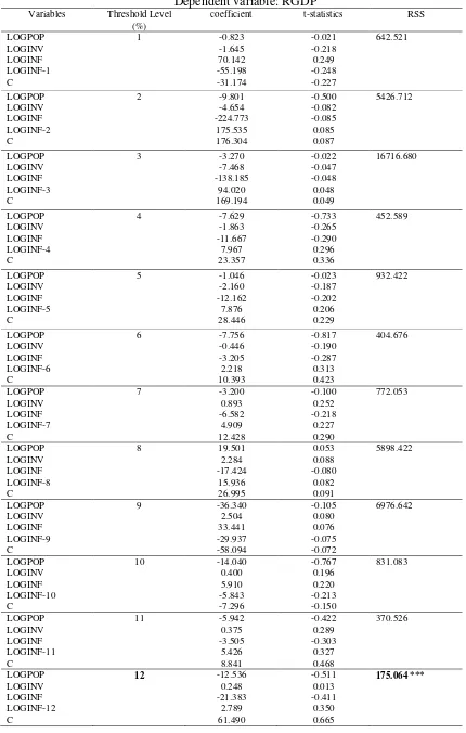
16 Table 6: 2SLS threshold estimation results

Dependent variable: RGDP

Variables Threshold Level (%)

coefficient t-statistics RSS

LOGPOP LOGINV LOGINF LOGINF-1 C

1 -0.823

-1.645 70.142 -55.198 -31.174 -0.021 -0.218 0.249 -0.248 -0.227 642.521 LOGPOP LOGINV LOGINF LOGINF-2 C

2 -9.801

-4.654 -224.773 175.535 176.304 -0.500 -0.082 -0.085 0.085 0.087 5426.712 LOGPOP LOGINV LOGINF LOGINF-3 C

3 -3.270

4 -7.629

5 -1.046

6 -7.756

7 -3.200

0.893 -6.582 4.909 12.428 -0.100 0.252 -0.218 0.227 0.290 772.053 LOGPOP LOGINV LOGINF LOGINF-8 C

8 19.501

2.284 -17.424 15.936 26.995 0.053 0.088 -0.080 0.082 0.091 5898.422 LOGPOP LOGINV LOGINF LOGINF-9 C

9 -36.340

2.504 33.441 -29.937 -58.094 -0.105 0.080 0.076 -0.075 -0.072 6976.642 LOGPOP LOGINV LOGINF LOGINF-10 C

10 -14.040

0.400 5.910 -5.843 -7.296 -0.767 0.196 0.220 -0.213 -0.150 831.083 LOGPOP LOGINV LOGINF LOGINF-11 C

11 -5.942

0.375 -3.505 5.426 8.841 -0.422 0.289 -0.303 0.327 0.468 370.526 LOGPOP LOGINV LOGINF LOGINF-12 C

12 -12.536

(18)

17

LOGPOP LOGINV LOGINF LOGINF-13 C

13 13.665

-1.883 -48.179

6.428 135.940

0.067 -0.105 -0.117 0.117 0.120

2863.406

Notes:*/**/*** statistically significant at 10%, 5%, 1% ** RSS at minimum value

Instrument specification: RGDP(-1) LOGPOP LOGINV LOGINF

Table 6 present the results for 2SLS. To examine the robustness of the estimated inflation

threshold level this study re-estimate equation (5) for the period 1980 to 2015. The purpose of

estimating 2SLS is in order to avoid possible specification bias of estimations. Similarly, results

from 2SLS are consistent with those of OLS estimation. It can be observed in the table that the

optimal threshold level is 12%, which is determined where RSS is at minimal point. At this

level it means that if Swaziland inflation level is beyond 12%, it will negatively impact

economic growth by -18.59% = (2.789 - 21.383). The study also applied the diagnostic tests

for only the equation that provides an optimal inflation level. However, only few tests were

conducted (see Appendix 2).All the test carried out satisfied the assumptions of classical liner

regression.

5. Conclusion

The main objective of this study was to estimate optimal threshold effect of inflation in

Swaziland. Firstly, the study performed the preliminary analysis such as unit root testing,

correlation analysis and pairwise granger causality analysis. The causality results indicated that

causality is running from inflation to economic growth. The study used liner approach of OLS

and 2SLS for the period 1980 to 2015 to investigate the threshold between inflation and

economic growth. In application of OLS the study found that the optimal threshold point is

[image:18.595.72.500.71.133.2]

(19)

18 robustness results were also attained in applying 2SLS method, which indicates negative

inflation effect beyond threshold point by 18.5%. In both estimation techniques, they were

subject to diagnostic tests and results shown no sign of violation of liner regression

assumptions. The determination of threshold level of 12% is consistent with work done by

Mkhatshwa, Tijani and Masuku (2015). In addition, this optimal threshold of 12% was

relatively estimated by the study of Khan and Senhadji (2000) for developing countries.

These findings on Swaziland economy may have crucial implications for monetary policy

makers in terms of keeping inflation below the threshold level point to sustain a positive

economic growth in the long run. The recommendation to monetary policy makers in

Swaziland is to carefully reconsider the monitoring of inflation for Swaziland, which is directly

driven by South African Reserve Bank (SARB) authorities through Common Monetary Area

(CMA) agreement. The target for SARB is to sustain inflation between 3% and 6%, hence the

upper band 6% is if far low compared to estimated 12% for conducive economic growth for

Swaziland.

References

Alkahtani, S.H. and Elhendy, A.M. (2014). Optimal inflation rate estimation for the Kingdom of Saudi Arabia: a threshold model approach. Life Science Journal, 11(4): 73-78.

Bawa, S. and Abdullahi, I.S. (2012). Threshold effect of inflation on economic growth in Nigeria. Journal of Applied Statistics, 3(1): 43 - 63.

(20)

19 Biswas, B.P. Masuduzzaman, M. and Siddique, M.N. (2016). Determining the

growth-maximizing threshold level of inflation in Bangladesh. Research Department Bangladesh Bank, Working Paper Series, WP No. 1602.

Dickey, D.A. and Fuller, W.A. (1970). Likelihood ratio statistics for autoregressive time series with a unit root. Econometrica, 49(4): 1057–1072.

Friedman, M. (1956). The quantity theory of money - a restatement. In M. Friedman (Ed), Studies in the quantity theory of money. Chicago: University of Chicago Press.

Hasanov, F. (2011). Relationship between inflation and economic growth in Azerbaijani economy: is there any threshold effect? Munich Personal RePEc archive paper no. 33494.

Makuria A.G. (2013).The relationship between inflation and economic growth in Ethiopia. (Unpublished Master thesis). Pretoria: University of South Africa.

Marbuah, G. (2010). The inflation-growth nexus: testing for optimal inflation for Ghana. Journal of Monetary and Economic Integration, 11(2): 71-72.

Mkhatshwa, Z.S., Tijani, A.S. and Masuku, M.B. (2015). Analysis of the relationship between inflation, economic growth and agricultural growth in Swaziland from 1980-2013. Journal of Economics and Sustainable Development, 6(18): 189-204.

Quartey, P. (2010). Price stability and the growth maximizing rate of inflation for Ghana. Modern Economy, 1: 180-194.

Romer, P. (1990). Endogenous technological change. Journal of Political Economy, 98: S71-S102.

Rutayisire, M.J. (2013). Threshold effects in the relationship between inflation and economic growth: evidence from Rwanda. AERC Research Paper 293. Nairobi: African Economic Research Consortium.

Sala-i-Martin, X. (1997). I just ran two million regressions. American Economic Review, 87(2): 178-183.

(21)

20 Sindano, A. (2014). Inflation and economic growth: an estimate of an optimal level of inflation

in Namibia (Unpublished master thesis). Windhoek: University of Namibia,.

Solow, R.M. (1956). A contribution to the theory of economic growth. The QuarterlyJournal of Economics 70(1): 65 - 94.

United Nations Economic Commission for Africa. (2016). Country profile – Swaziland. Addis Ababa: United Nations Economic Commission for Africa.

Vinayagathasan, T. (2013). Inflation and economic growth: a dynamic panel threshold analysis for Asian economies. Journal of Asian Economies, 26: 31 – 41.

Yabu, N. and Kessy, N.J. (2015). Appropriate threshold level of inflation for economic growth: evidence from the three founding EAC countries. Applied Economics and Finance, 2(3): 127 -144.

Younus, S. (2012). Estimating growth-inflation trade-off threshold in Bangladesh. Bangladesh Bank Working Paper, Dhaka: Bangladesh Bank.

Appendix 1: OLS estimation diagnostic test results

Diagnostic Test Test statistics (p-value)

conclusion

Normality

(Jarqua-Bera test)

0.357 (0.836)

Residual are normally distributed

Serial correlation

(Breusch-Godfrey LM Test)

1.477 (0.477)

No serial correlation