The interplay between problem loans and Japanese bank productivity

Munich Personal RePEc Archive

The interplay between problem loans and

Japanese bank productivity.

Mamatzakis, Emmanuel and matousek, roman and vu, anh

University of Sussex Business School

14 March 2019

The interplay between problem loans and Japanese bank productivity.

Emmanuel Mamatzakisa_{, Roman Matousek}b _{and Anh Nguyet Vu}c

March 2019

Abstract

This paper examines for the first time the impact of problem loans on Japanese productivity growth. We exploit a new data set of Japanese problem loans classified into two categories: bankrupt and restructured loans. We opt for a novel and flexible productivity growth decomposition that allows to measure the direct impact of these problem loans on productivity growth. The results reveal that Japanese bank productivity growth was severely constrained by bankrupt and restructured loans early in 2000s, whilst some persistence of the negative impact of problem loans on productivity growth is observed in the late 2000s. Thereafter, there is only some partial recovery in the productivity growth from 2012 to 2015. Further, we also perform cluster analysis to examine convergence or divergence across regions and over time. We observe limited convergence, though Regional Banks seem to form clusters in some regions.

Keywords: Bank productivity; Bankrupt loans; Restructured loans; Cluster analysis; Japan.

JEL classification: D24, G21, C33

a_{University of Sussex, School of Business, Management and Economics, Falmer, Brighton, BN1 9SL,}

United Kingdom. b_{Nottingham University Business School, Nottingham NG8 1BB, United Kingdom.}

Email address: Roman.Matousek@nottingham.ac.uk. c_{University of Sussex, School of Business,}

1

1. INTRODUCTION

There has been extensive theoretical and empirical research into the field of firm efficiency

and productivity (Heshmati, Kumbhakar, & Sun, 2014; Subal C. Kumbhakar & Tsionas, 2016; Sun, Kumbhakar, & Tveterås, 2015). In terms of bank efficiency and productivity, the outbreak

of the global financial crisis has driven a surge of banking studies (Matousek, Rughoo, Sarantis, & Assaf, 2015; Tsionas, Assaf, & Matousek, 2015;, Mamatzakis et al. 2016; Mamatzakis and Tsionas, 2019), unfolding the paramount importance of financial intermediaries within the

economic system. In terms of productivity growth, evidence is rather limited with studies that apply parametric methods to evaluate bank productivity (Boucinha, Ribeiro, & Weyman-Jones,

2013; Feng & Serletis, 2010; Feng & Zhang, 2012, 2014). As indicated in a review of non-parametric productivity applied in banking by Fethi and Pasiouras (2010), the majority of studies adopt a non-parametric approach (Fukuyama & Weber, 2005, 2010; Liu & Tone, 2008).

Our study extends the literature on bank productivity by opting for a parametric estimation technique. We decompose bank productivity growth into different components, namely the effects of problem loans, which are essentially uncontrollable inputs, quasi-fixed input, returns

to scale, and technological change. The Japanese banking system is of interest as its performance has been undermined by an unprecedented volume of bankrupt and restructured

loans. These loans are referred as risk-monitored loans disclosed in accordance with the Japanese Banking Law. Moreover, in Japanese banking literature, bank efficiency studies have

dominated the research field of bank performance, for example Drake and Hall (2003), Fukuyama and Weber (2005), Fukuyama and Weber (2010), Barros, Managi, and Matousek (2012), Yang and Morita (2013). Japanese bank productivity has been rather neglected (Assaf,

2

We, thus, fill a gap in the literature and apply for the first time a productivity growth decomposition to Japanese banks, where problem loans’ impact would be revealed.1 _Previous

literature has considered nonperforming loans as uncontrollable inputs or undesirable outputs in the banking production process (Assaf, Matousek, & Tsionas, 2013; Barros et al., 2012;

Drake & Hall, 2003; Fukuyama & Weber, 2008; Glass, McKillop, Quinn, & Wilson, 2014; Hughes & Mester, 2010; Mamatzakis, Matousek, & Vu, 2016; Mamatzakis and Vu 2018; Mamatzakis and Tsionas 2017). We follow Drake and Hall (2003) and Hughes and Mester

(2010) to treat bankrupt and restructured loans as uncontrollable inputs in our productivity decomposition.2 _{Given the extensive volume of bankrupt and restructured loans in Japan, we}

expect that they have an impact on bank productivity. Arguably, banks may receive payments of the principal and interest on these loans subject to borrowers’ financial health. These overdue

loans in turn would raise bank’s operating costs in the short-run. Hence, one would expect these

loans to deteriorate bank productivity.

Alongside bankrupt and restructured loans, we also employ equity as a quasi-fixed input (Berger & DeYoung, 1997; Hughes, Mester, & Moon, 2001; Ray & Das, 2010; Mamatzakis

and Bermpei 2016; Mamatzakis et al. 2015). Within a short period, it would be unfeasible to adjust the level of equity considerably and quickly (Lozano-Vivas & Pasiouras, 2014;

Mamatzakis and Tsionas, 2019; Mamatzakis and Tsionas, 2017; Mamatzakis and Koutsomanolis-Filippaki, 2009). In the event of unexpected losses, the level of equity is of

utmost importance to ensure bank safety and soundness, preventing banks from temporary illiquidity and insolvency (Diamond & Rajan, 2000; Mamatzakis and Koutsomanolis-Filippaki, 2009). Equity would also serve as a cost-reducing factor due to less interest paid for debt

financing (Hughes & Mester, 2013; Mamatzakis and Psillaki 2017). Finally, the inclusion of equity in our productivity decomposition is of importance for Japan. The reason is that during

3

the early 2000s. The Japanese authorities responded by injecting public capital four times between March 1998 and June 2003 (Hoshi & Kashyap, 2010), hoping to stabilise the financial

market and revive the banking industry.

The contribution of this study can be summarised in the following ways. First, we expand

the parametric methodological literature of bank productivity growth (Boucinha et al., 2013; Casu, Ferrari, & Zhao, 2013; Lozano-Vivas & Pasiouras, 2014) as opposed to the broadly applied nonparametric one (Alam, 2001; Berg, Forsund, & Jansen, 1992; Delis, Molyneux, &

Pasiouras, 2011; Fiordelisi & Molyneux, 2010; Grifell-Tatjé & Lovell, 1997; Kao & Liu, 2014; Wheelock & Wilson, 1999). Our paper refers to Japan, which serves as an excellent case study

given the trouble of its banking industry (Barros, Managi, & Matousek, 2009; Fukuyama, 1995; Fukuyama & Weber, 2002). Second, we exploit a new data set of bankrupt and restructured loans, which are disaggregated from “risk-monitored loans” disclosed subject to the Japanese

Banking Law. The adopted approach enables a comprehensive analysis by allowing for the impact of these loans on total factor productivity growth. Finally, we test for convergence – catching up effect – among Japanese banks and geographic regions by using club convergence

analysis proposed by Phillips and Sul (2007). This methodology is superior compared to others

such as the β-convergence and σ-convergence. For a panel data variable, it can detect

convergence in sub-groups even though convergence is rejected at the whole panel level. After

more than a decade of the banking crisis and structural reforms, converging on productivity growth would indicate that Japanese banks have been brought together to facilitate further necessary policy changes, especially on the ground of continued deflation and low economic

growth (Mamatzakis E and F Avalos 2018; Mamatzakis and Vu 2018).

Our results show that productivity growth in Japanese commercial banks is impaired by

4

to capture events such as government interventions, the global financial crisis, and the Tohoku tsunami/earthquake. Interestingly, restructured loans are among the drivers of productivity

growth, as they are found to lower costs. With regard to the club convergence analysis, we find divergence in productivity growth across regions over time. However, some integration, and

thus convergence, is identified for Regional Banks I, whereas there exist some clubs of convergence within City Banks, and within the regions of Hokkaido, Tohoku, Kanto, Chubu, Chugoku, and Shikoku.

The remainder of this paper is structured as follows. Section 2 provides an overview of the literature in bank productivity. Section 3 presents the methodology, followed by the data

description in section 4. Empirical results are provided in section 5, and convergence tests are discussed in section 6. Finally, section 7 concludes.

2. LITERATURE REVIEW

This section highlights the literature in bank productivity with a particular focus on the approaches used to decompose total factor productivity (TFP) growth. In what follows, we briefly survey the studies that apply nonparametric and parametric methodologies to measure

bank productivity.

2.1. Non-parametric studies

The decomposition of the Malmquist productivity index through Data Envelopment Analysis (DEA) has prevailed in the banking literature. As indicated in a comprehensive review

for bank efficiency and productivity (Fethi & Pasiouras, 2010), almost all studies before 2010 apply this approach. Berg et al. (1992) use this technique to obtain the productivity index for Norwegian banking, where the largest banks are found to be strongly productive after

Grifell-5

Tatjé and Lovell (1997) replace the Malmquist productivity index by a generalised Malmquist productivity index, allowing for the measurement of the contribution of scale economies on

productivity growth. In a similar vein, Fiordelisi and Molyneux (2010) obtain TFP growth of European banking, where technological change was the most productive component which contributed to shareholder’s value. Other studies include Tortosa-Ausina, Grifell-Tatjé,

Armero, and Conesa (2008), which use a bootstrapping techniques to derive the Malmquist index, and Kao and Liu (2014), which employ a probabilistic analysis. Productivity growth

studies in Japanese banking are also dominated by those adopting nonparametric methodologies (Assaf et al., 2011; Barros et al., 2009; Fukuyama, 1995; Fukuyama et al., 1999;

Fukuyama & Weber, 2002).

Flexibility is the main feature of a semi-parametric approach that attracts research interest. This methodology to measure productivity, however, has been mainly applied in nonbanking

research (Heshmati et al., 2014). Sun et al. (2015) propose a semiparametric cost frontier of which the slope coefficients are a nonparametric function of the time trend. The semiparametric cost function is estimated first, followed by a decomposition of inefficiency into time-varying

and time-invariant components. Finally, productivity is decomposed based on the estimated cost frontier. Although the authors use Norwegian farming data set as an example, this

methodology could also be of interest for banking applications.

2.2. Parametric studies

Bank productivity in parametric studies is mainly derived from estimating cost, profit, or distance functions. For the use of the cost function, Kim and Weiss (1989) estimate an equation system consisting of the translog cost function and cost shares of inputs to examine the effect

of branches on TFP growth of Israeli banks during 1979-1982. For the Indian banking sector from 1985 to 1996, Kumbhakar and Sarkar (2003) estimate a translog shadow cost function

6

regression. TFP growth is decomposed into three components: a scale factor, a technological change, and a miscellaneous part. All three factors depend on regulation via shadow prices of

inputs which are a product of actual input prices and a function component defined as the distortion function of labour relative to capital. Also utilising the cost function, Stiroh (2000)

examines productivity in US bank holding companies during the 1990s using several econometric approaches: i) pooling annual data and estimate the shift from the cost function; ii) incorporating bank holding companies’ specific effects in panel data, and estimating the

shift in a common cost function; and iii) decomposing total cost changes into changes in business conditions and in productivity. Estimating a cost function on its own by using

stochastic frontier analysis, Boucinha et al. (2013) obtain the estimated parameters and compute total factor productivity change for Portuguese banks. Their results suggest that technological progress was the main driver of total factor productivity change from 1992 to

2006.

Berger and Mester (2003) estimate cost and profit functions for US banks during 1991-1997 to obtain cost productivity change and profit productivity change. Productivity change in

this study is defined as changes in best practice and changes in inefficiency. Focusing on off-balance sheet variables, Lozano-Vivas and Pasiouras (2014) also obtain productivity change

by applying this parametric decomposition on an international sample for the period 1999-2006. Using a translog profit function, Kumbhakar, Lozano-Vivas, Lovell, and Hasan (2001)

measure productivity change as the sum of technical change which is defined as shifts in the profit frontier, and variation in the components of profit technical efficiency. For Spanish saving banks during 1986-1995, there was evidence for high technical inefficiency, but

significant technical progress. Following the parametric technique in Berger and Mester (2003), Casu, Girardone, and Molyneux (2004) obtain productivity growth of European

7

strong productivity growth for Italian and Spanish banks, whereas mixed evidence is reported for the German and French banking sectors. Casu et al. (2013) also use both Data Envelopment

Analysis (DEA) and Stochastic Frontier Analysis (SFA) to estimate productivity change of Indian banks 1992-2009. They further conduct a metafrontier analysis to account for

technology heterogeneity amongst banks with different ownership structures.

Chaffai, Dietsch, and Lozano-Vivas (2001) use a stochastic output distance function to decompose the Malmquist index into pure technological effect and environmental effect. Orea

(2002) also opts for the distance function to introduce a parametric decomposition of a generalised Malmquist productivity index. The TFP index in Orea (2002) is contributed by the

Malmquist productivity index and a returns to scale term. Applying the parametric decomposition for Spanish saving banks (1985-1998), Orea (2002) finds that TFP growth was mainly attributed to technical progress, although the scale effect also revealed a positive impact

on productivity change. Koutsomanoli-Filippaki, Margaritis, and Staikouras (2009) parameterise the directional distance function to examine Luenberger productivity indicator for banking industries in Central and Eastern European countries (1998-2003). Their finding

suggests that the dominant factor driving productivity growth was technological change. Feng and Zhang (2012) and Feng and Zhang (2014) adopt a true random stochastic distance frontier model to allow for unobserved heterogeneity among US banks. The “output

-distance-function-based-Divisa” productivity index proposed in Feng and Serletis (2010) is used in these studies

to measure TFP growth of large US banks.

3. METHODOLOGY

3.1. Decomposing productivity growth

8





=



=min : ( , , , , ) 0

) , , , ,

(wY b E t wX F X Y b E t C

X (1)

or k

K k kX w C



=  1 (2)

where F denotes the production function with outputs Y, inputs X, input prices w (with k being

the number of inputs), input b which is outside the control of the bank, equity E, and technology

t. We treat equity E as quasi-fixed as adjustment in equity quickly is over the long run (Lozano-Vivas & Pasiouras, 2014).

To derive the impact of bank input outside the control of the bank (i.e. problem loans) on

productivity growth, we adopt the methodology proposed by Morrison and Schwartz (1996). Thus, total differentiating equation (1) with respect to time yields:

t C t E E C t b b C t Y Y C t w w C dt

dC J j

j j m M m m k K

k k 

 +     +     +     +     =







= =

=1 1 1

(3)

Dividing both sides of equation (3) by total cost C, we obtain:

t C C E E E C C b b b C C Y Y Y C C w w w C C C dt dC j j j J j m m m M m k k k K k   +   +   +   +   =   =  =  =







1 1 1 1 1 (4) where k k k w t w w 1   =  ; m m m Y t Y Y 1   =  ; j j j b t b b 1   =  ; E t E E 1   = 

; k K

C X w w w C C

S k k

k k

k _  , =1,...,

 =

being the cost share of bank input k; m M Y Y C C m m

CYm  , =1,...,

 =

 being the cost elasticity with

respect to output m; j J b b C C j j

Cbj  , =1,...,

 =

 being the cost elasticity with respect to

uncontrollable input j;

E E C C CE _  =

 being the cost elasticity with respect to equity; and

t C C Ct _  = 1

 being the technical change. 3

Thus, we can obtain equation (5), where

dt dC C=



9 Ct CE j J j Cb m M m CY k K k

k w Y b E

S C

C

j

m   

 + + + + =   =  =  = 







1 1 1 (5)

Rearranging equation (5) with respect toCt , we get:

  =  =  =  − − − −

=



S w



Y



b E

C C CE j J j Cb m M m CY k K k k

Ct  m  j 



1 1

1

(6)

Thus, substituting the first two terms in the right-hand side of equation (6) with the term 4

as in equation (f.4.4) of footnote 4, we obtain equation (7):

  =  =  = − − −

=



X



Y



b E

C X w CE j J j Cb m M m CY k K k k k

Ct  _m  _j 



1 1

1

(7)

Now note that the total factor productivity growth (if constant returns to scale,_CY =1),

that is the Solow residual, showing the difference between the rate of change of outputs and

the rate of change of inputs is:

 = =  





−

= K _k

k k k M m m X C X w Y TFP 1 1 (8)

In the case of non-constant returns to scale, the traditional measure of productivity growth

will be adjusted by combining equations (7) and (8) to get:

  =  =  =  − − − −

=



Y TFP



Y



b_{j CE}E

J j Cb m M m CY M m m

Ct  m  j 



1 1

1

(9)

Rearranging equation (9), we obtain equation (10):

(

)

  =  =  − − − + −

=



Y



b E

TFP _{j CE}

J j Cb m M m CY

Ct  _m  _j 



1 1

1 (10)

The terms in the right-hand side of equation (10) are the impact of technological change, the scale effect, the impact of bank input outside the control of the bank (bankrupt and

10

3.2. The translog function

The specification of our translog cost function is as follows5_:

                      + + + + + + + + + + + + + + + + + + + + + =































= = = = = = = = = = = = = = = = = = = = = Et t b t Y t w t t E b E Y b Y E w b w Y w E E b b Y Y w w E b Y w C t j J j jt m M m mt k K k kt tt t J j j j m M m m j m M m J j mj k K k k j k K k J j kj m k K k M m km e s j J j S s js n m M m N n mn l k K k L l kl j J j j m M m m k K k k ln ln ln ln 2 1 ln ln ln ln ln ln ln ln ln ln ln ln ln ln 2 1 ln ln 2 1 ln ln 2 1 ln ln 2 1 ln ln ln ln ln 1 1 1 2 1 1 1 1 1 1 1 1 1 1 1 1 1 1 1 1 1 1 0 (11) where wk, Ym, bj, E denote kth _{input price, m}th _{output, j}th _{uncontrollable input, and equity}

respectively.

Applying Shephard’s lemma for equation (11), we obtain the shares of cost attributed to

input price kth_:

t E b Y w w

S _{j k kt}

J j kj m M m km l L l kl k kk k

k = + +



 +



 +



 + +

= = = ln ln ln ln ln 1 1 1 (12)

Total differentiating equation (11) with respect to output mth_{, uncontrollable input j}th_{, and} equity, we obtain:

t E b

w Y

Y _{j m mt}

J j mj k K k km n N n mn m mm m

CYm       

 = + +



+



+



+ + = = = ln ln ln ln ln 1 1 1 (13) t E Y w b

b _{m j t}

M m m k K k k s S s js j jj j

Cbj       

 = + +



+



+



+ + = = = ln ln ln ln ln 1 1 1 (14) t b Y w

E _{j t}

J j j m M m m k K k k e

CE      

11

The cost function requires a monotonic condition of non-decreasing in w. We impose the

usual symmetry restrictions kl =lk,mn =nm,js =sj and linear homogeneity restriction

on the cost function (11) with respect to input prices:

0 ; 0 ; 0 ; 0 ; 0 ; 1 1 1 1 1 1 1 = =  =  =  = =













= = = = = = K k kt K k k K k kj K k km K k kl K k

k  l  m  j  

 (16)

There are two input prices: price of fund, and price of physical capital and labour.6 _We

estimate equation (11) by using the price of fund to normalise. The results obtained are then

used to compute the impact of each component on productivity growth.

4. DATA

This paper employs a new data set of problem loans in Japan, providing new information of a critical bank uncontrollable input. Moreover, we disaggregate problem loans disclosed in

accordance with the Japanese Banking Law into two categories. The first one consists of loans to borrowers in legal bankruptcy, and past due loans in arrears by six months or more. The second component comprises loans in arrears by 3 months or more but less than 6 months, and

restructured loans. For simplicity, we name these two types of problem loans as bankrupt loans (BRL) and restructured loans (RSL) thereafter. Such disaggregation of problem loans has not

been employed widely in the Japanese banking productivity literature (Mamatzakis et al., 2016). This disaggregation allows us to explore the extent to which each uncontrollable input,

namely bankrupt loans and restructured loans, affects bank productivity.

In the aftermath of the asset price bubble that burst late 1990s in Japan, problem loans rose dramatically since a vast number of firms went bankrupt or experienced business difficulties.

The cost of bankrupt and restructured loans in 1997 was 30 trillion JPY (Hoshi & Kashyap, 2000). However, some sources estimate the actual value in excess of 100 trillion JPY (Hoshino,

12

medium-sized firms (SMEs) in order to ease the “credit crunch” (Hoshi, 2011; Hoshi & Kashyap, 2010). However, the fact that the government subsidised these unprofitable

borrowers dampened the entry and investment of productive firms, leading to fewer good lending opportunities for solvent banks (Caballero, Hoshi, & Kashyap, 2006). Prior to 2002,

the government had deployed rescue schemes by injecting capital and bailing out troubled banks, but it had been claimed that there were delays of much-needed restructuring at the banking industry (Caballero et al., 2006). Furthermore, misdirected bank lending augmented

the accumulated level of bankrupt and restructured loans. In 2002, the level of these loans fell, reflecting the effort of banks to reduce problem loans under the reform program introduced by

Heizo Takenaka, who was in charge of the Financial Services Agency. After the recovering period, the global financial crisis 2007-2008 somewhat increased further the level of bankrupt and restructured loans.

We employ a unique semi-annual data set provided by the Japanese Bankers Association. Our panel data consist of 3484 observations for Japanese commercial banks - 10 City Banks, 65 Regional Banks I, and 56 Regional Banks II - from financial years 2000 to 2014. City Banks

are the largest banks amongst the three types. Apart from conventional banking activities, their operation spreads widely from security investment to ancillary services (Tadesse, 2006).

Regional Banks, in contrast, strongly commit to the local development in their scope of business. They cater the financial need of SMEs within their geographic regions. Regional

Banks II are the smallest with a more prefectural focus.

To define outputs and input prices, we follow the widely accepted intermediation approach (Sealey & Lindley, 1977). In our cost function, in line with Fukuyama and Weber

(2009), Barros et al. (2012), Assaf et al. (2011), we specify two outputs: y1 net loans and bills discounted, and y2 earning assets which include investments, securities, and other earning

13

obtain their share from noninterest expenses. Therefore, we define two input prices: price of fund, and price of physical capital and labour, in line with Fu, Lin, and Molyneux (2014). Price

of fund w1 is the ratio of interest expenses divided by total deposits and borrowed funds. Price of physical capital and labour w2 is the ratio of noninterest expenses divided by fixed assets.

Equity is included in the cost function as a quasi-fixed input (Hughes & Mester, 2013). Table 1 describes the summary statistics of key variables in our panel data.

[INSERT TABLE 1 ABOUT HERE]

5. EMPIRICAL RESULTS

5.1. Cost elasticities with respect to uncontrollable inputs and equity

Estimated parameters satisfy the monotonic condition and linear homogeneity constraints of the cost function.7 _{The coefficients are statistically significant with appropriate signs as}

expected. Bankrupt loans are found to have a slightly stronger impact on cost than restructured loans (the parameters are 0.0384 and 0.0203 respectively). The impact of equity on cost is

positive and significant (0.0533). We report the elasticities of cost with respect to bankrupt loans, restructured loans, equity and outputs in Table 2. Overall, for all banks in the sample, these variables expose a cost-augmenting effect. The average cost elasticities with respect to

bankrupt loans, restructured loans, and equity are reported at 0.0385, 0.0201, and 0.0537 respectively. In sub-periods, while the cost elasticity with respect to bankrupt loans appears to

vary over time, the cost elasticity with respect to restructured loans decreases monotonically, turning out negative in the last two sub-periods (-0.0002 and -0.0106). This negative cost

elasticity is attributed to the negative values found for City Banks and Regional Banks I. In terms of equity, there is variability in cost elasticities. The largest magnitudes for cost elasticities with respect to equity are in the first two sub-periods, 0.0721 in September

14

equity prevailing during the acute phase of the banking crisis and the restructuring period. Afterwards, the cost elasticity with respect to equity declines to 0.0415 in September

2006-March 2009, and thereafter, further down to 0.0194 in September 2009-2006-March 2012. This finding is in line with King (2009). King (2009) reports that the magnitude of the cost of equity

incurred by Japanese banks is higher compared to that in other countries such as Canada, France, Germany, UK, and US.

[INSERT TABLE 2 ABOUT HERE]

Breaking up the cost elasticities according to bank types, we observe a decreasing trend of the cost elasticities with respect to uncontrollable inputs for City Banks. Note that these values

are negative in the case of restructured loans in all sub-periods and in the case of bankrupt loans during the September 2012-March 2015 period. For Regional Banks I and II, there is also a downward trend for the cost elasticities with respect to restructured loans. In the September

2009-March 2012 period and September 2012-March 2015 period, there are negative cost elasticities with respect to restructured loans in Regional Banks I. These findings show that restructured loans do not always raise cost. This is an interesting finding which could indicate

that changes in legislation to restructure the industry might have been effective. A component of our restructured loan data relates to loans of which interest rates have been lowered, contracts

have been amended, and/or loans to corporations under ongoing reorganisation (Montgomery & Shimizutani, 2009). Without this process, these loans would be more likely to become

nonperforming loans, raising further bank costs. Other government support measures include the Act on Special Measures for Strengthening Financial Functions (August 2004-March 2008, December 2008) and the SME Financing Facilitation Act (2008-2013) (Hoshi & Kashyap,

2010; Endo, 2013). These Acts include capital injection programs, the relaxation of capital adequacy requirements, and changes in the regulatory framework which allowed bad loans of

15

Apart from government support measures, the nature of business might also explain for the cost-saving impact of restructured loans. Regional Banks are committed to the development of

the local regions where their headquarters are situated. SMEs are among their target clients. Therefore, Regional Banks are motivated to support SMEs through amending bad loans. As a

result, 3-6% total credit was reclassified under the SME Financing Facilitation Act (International Monetary Fund, 2012).8

Another noteworthy finding is the cost-saving impact of equity for City Banks, on average at -0.0221. While the cost elasticity with respect to equity remains positive in all sub-periods

for Regional Banks I and II, it is positive only in September 2003 to March 2006 for City Banks. Hence, equity financing might benefit City Banks in terms of mitigating the interest burden from debt financing, supporting the argument of Hughes and Mester (2013). Note that

City Banks also received support from public capital during the restructuring process, thus benefiting from the rescue capital. These negative elasticities could also be interpreted as how

much banks are willing to pay for equity as it would result in cost saving (Boucinha et al., 2013). Boucinha et al. (2013) also report a desirable impact of equity in lessening costs for Portuguese banks during 1992-2006. In contrast, this may not apply for Regional Banks. Their

cost elasticities with respect to equity appear to have variability over time, with a more pronounced magnitude in Regional Banks I (0.0608) than in Regional Banks II (0.0541).

The average cost elasticity with respect to outputs for all banks is 0.636 (which is less than 1 so scale economies exist). Overall, there is an upward trend of the average cost elasticity with

respect to outputs over time, starting from 0.563 in the first period to 0.722 in the last sub-period. In particular, City Banks experience decreasing returns to scale (1.025), while Regional Banks benefit from increasing returns to scale (0.652 for Regional Banks I and 0.561 for

16

2014). The cost elasticities with respect to outputs vary over time for City Banks, with the second sub-period (September 2003 – March 2006) recording the lowest average value at

0.932. The cost elasticities with respect to outputs for both types of Regional Banks, in contrast, are less volatile than those of City Banks.

5.2. Total factor productivity growth over time

In Table 3, we report the average values (semi-annually) of TFP growth over time. On

average, the productivity growth of Japanese banks during the years 2000-2014 is at 0.52%. In the first sub-period March 2001-March 2003, Japanese banks experienced negative

productivity growth, which could be expected since they were undergoing major reforms to restore financial stability post-crisis. In the second sub-period September 2003-March 2006, TFP exhibited a strong growth at an average of 1.37%, thanks to the decline in bankrupt loans

and restructured loans. This could also be attributed to the effect of quantitative easing in stimulating economic activity (Girardin & Moussa, 2011).9 _{In the third sub-period September}

2006-March 2009, TFP growth dropped markedly to 0.27%, possibly because of the onset of the global financial crisis 2007-2008. The destructive effect of the crisis seems short-lived, as TFP growth bounced back to 1.09% during the September 2009-March 2012 period, followed

by a decrease to 0.6% in the last sub-period September 2012-March 2015. With reference to the Japanese banking literature, there are a few studies which estimate bank productivity

growth, though not very recent. Using the indirect Malmquist–Russell productivity index, Fukuyama and Weber (2002) report a 2% decline per year on average for Japanese banks

operating between 1992 and 1996. Studying Japanese credit cooperative banks and using the bootstrapped Malmquist index, Assaf et al. (2011) find that their productivity growth did not rise significantly during 2000-2006. Fukuyama and Weber (2017) is the latest study examining

2007-17

2012 in their study is similar to our finding. Their dynamic network Luenberger indicator of productivity growth was increasing for the observed period.

[INSERT TABLE 3 ABOUT HERE]

Among bank categories, City Banks were the most productive, on average at 1.12%,

followed by Regional Banks I (0.65%). The smallest banks in size, Regional Banks II, performed the lowest growth of 0.26% on average. This is in line with findings of Fukuyama and Weber (2017). Fukuyama (1995) also reports that between 1989 and 1991, City Banks

were more productive than Regional Banks. In a similar vein, Barros et al. (2012) find that City Banks were the most efficient among the three types during 2000-2007. During the

restructuring and the first quantitative easing period (March 2001-March 2006), City Banks experienced substantial growth in their productivity, notably at 2.32% during March 2001-March 2003 and 2.65% during September 2003-2001-March 2006. The other two types, in contrast,

underwent negative productivity growth in the restructuring period, -0.43% for Regional Banks I and -1.78% for Regional Banks II. Like City Banks, their productivity growth increased significantly during the initial quantitative easing period September 2003-March 2006 (1.4%

and 1.15%). In the third sub-period September 2006-March 2009, which covers the duration of the global financial crisis 2007-2008, City Banks bore a loss in productivity growth, -0.86%.

Fukuyama and Weber (2017) also report negative productivity growth for City Banks during 2007-2008. Productivity growth of Regional Banks also dropped to 0.17% (Regional Banks I)

and 0.57% (Regional Banks II). Afterwards, productivity growth rose to 2.93% in City Banks, 1.17% in Regional Banks I, and 0.74% in Regional Banks II. These results are relatively similar to the trend and the magnitude of change of productivity growth in Fukuyama and Weber (2017). Studying Regional Banks’ efficiency, Fukuyama and Matousek (2017) also report a

decreasing trend of technical inefficiency for Regional Banks I after the global financial crisis

18

last sub-period September 2012-March 2015, which embraced the aggressive quantitative easing time frame, witnessed a considerable decline in productivity growth of City Banks

(down to -2.17%). Other bank types also saw a fall in their productivity growth.

5.3. Total factor productivity growth decomposition

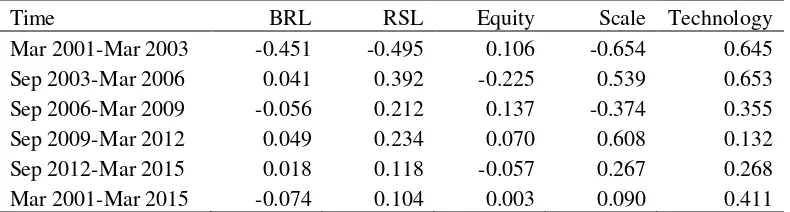
To shed light into the contribution of each component to TFP growth, we report the average values of the effect of each component in Table 4, according to equation (10) of our model. From March 2001 to March 2003, bankrupt loans dampened TFP growth by -0.45.

Nevertheless, their negative effect was smaller compared to the impact of restructured loans, -0.49, and the impact of returns to scale, -0.654. Equity and technological change positively

contributed to productivity growth by 0.11 and 0.65 respectively. In the second sub-period September 2003-March 2006, large productivity growth was a result of the decline in bankrupt and restructured loans, the rise in the scale effect, and technological progress.

[INSERT TABLE 4 ABOUT HERE]

In the third sub-period September 2006-March 2009, on average, bankrupt loans constrained productivity growth with a magnitude of -0.06. In contrast, from September 2009

onwards, they in fact contributed to productivity gain because there was a drop in the level of bankrupt loans for the whole banking system (gradually down from 8458 billion JPY in

September 2009 to 5896 billion JPY in March 2015). Using nonperforming loan ratio as a control variable in the cost function, Altunbas, Liu, Molyneux, and Seth (2000) find a positive

relationship between nonperforming loans and inefficiency. Mamatzakis et al. (2016) also report a negative impact of problem loans on Japanese bank performance. Like bankrupt loans, restructured loans had imposed a negative effect on TFP growth (-0.49) before the

19

contributing to productivity growth by 0.39%. From September 2006 to March 2015, the positive impact of restructured loans on TFP growth remained. Note that there was an increase

in restructured loans in the last two sub-periods. It could be the case that the US credit crunch imposed a destructive effect on Japanese bank productivity growth with a lag, which was

reflected in the rise of restructured loans after the crisis. The Tohoku-Pacific Ocean earthquake in March 2011, which has been the most powerful earthquake ever in Japan, might also be among the reasons for the rising of restructured loans afterwards.

Equity was among the growth drivers, although its average impact on productivity growth was small (0.003) for the whole sample period. In the initial sub-period March 2001-March

2003, 0.11% was the contribution of equity to TFP growth. This could stem from the fact that banks were undercapitalised post-crisis, and during that time of uncertainty, the cost of equity financing was high. Nevertheless, banks that failed to raise enough equity were eventually

rescued by public capital (Montgomery & Shimizutani, 2009). Therefore, they benefited from government subsidisation and could make use of the bailout capital. In the second and the last subperiods, equity put more weight on the cost burden, thus eroding productivity growth,

-0.23 during September 2003-March 2006 and -0.06 during September 2012-March 2015. Between September 2006 and March 2012, equity positively contributed to productivity

growth.

Overall, technical progress was consistently the driving force of TFP growth. Over the

whole period, technology accounted for the increase in TFP growth on average at 0.41. Tadesse (2006) also reports evidence for technological progress in Japanese banks between 1974 and 1991. The scale effect, although fluctuating over time, on average contribute to productivity

growth (0.09%). Boucinha et al. (2013) also find a significant contribution of returns to scale to increased productivity growth of Portuguese banks. Feng and Serletis (2010) find a moderate

20

0.44%. Yet, the scale effect is the second largest component (after technical change) of US banks’ productivity growth. Computing technical and scale efficiency for Japanese commercial

banks in 1990, Fukuyama (1993) reports that scale inefficiency is negligible compared to pure technical inefficiency. Regarding the quasi-fixed input, the magnitude of the contribution of

equity over time is not considerable, 0.003. In terms of uncontrollable inputs, bankrupt loans, on average, showed a detrimental impact on TFP growth, -0.07. Restructured loans, in contrast, was among the main driving forces for productivity growth, 0.104. There is evidence to support

that the increase in TFP growth during September 2003-March 2006 was partly attributed to the fall in bankrupt loans and restructured loans. The reverse is true for the initial sub-period,

when the loss in TFP growth was also mainly explained by the scale effect.

5.4. Total factor productivity decomposition per type of banks

Table 5 reports the decomposition of TFP growth for each bank type. In terms of the effects

of uncontrollable inputs, on average bankrupt loans exhibit a destructive effect on productivity growth of all banks. The magnitude of the impact is greater for City Banks, -0.23, than for Regional Banks I, -0.04, and Regional Banks II, -0.09. In the first sub-period March

2001-March 2003, except City Banks, Regional Banks suffered a damaging effect of bankrupt loans on TFP growth. This finding could indicate that the restructuring scheme had helped City

Banks to cut their bankrupt loan level. Afterwards, Regional Banks had to bear that impairment again during September 2006-March 2009. From September 2003-March 2015, City Banks

endured a negative impact of bankrupt loans on productivity growth. It could be that the global financial crisis worsened the likelihood of recovery of bankrupt loans and downgraded restructured loans to bankrupt loans. The effect could be more pronounced in City Banks than

in the others because of their size and business structure. Regional Banks are more geographical focus, thus, were less exposed to the contagion effect of the US credit crunch.

21

Restructured loans appear beneficial to productivity growth of each bank type. On average, they contributed to TFP growth of all types, more considerably for City Banks, 0.33. Yet, City

Banks had to face a negative effect of restructured loans from September 2003 to March 2009. In the initial sub-period, Regional Banks suffered from an adverse effect of restructured loans

on their productivity growth, while the contrary is reported for City Banks. In the remaining sub-periods, restructured loans enhanced TFP growth of Regional Banks. In terms of equity, on average, equity undermined productivity growth of Regional Banks II by -0.05, while the

effect is favourable for City Banks, 0.21, and Regional Banks I, 0.02. Over time, there was a volatile impact of equity on productivity growth of Regional Banks I. From September 2003

to March 2015, the impact of equity was persistently negative for Regional Banks II, but positive for City Banks. As aforementioned, the majority of City Banks and some Regional Banks were recipients of public funds (Hoshi and Kashyap, 2010). We could not rule out the

potential benefits from capital injection programs as well as the impact of equity in saving interest costs from debt financing (Hughes and Mester, 2013).

Regarding the scale effect, the influence of the global financial crisis on all banks could be

reflected in our results. The reason is that the contribution of returns to scale declined considerably in the third sub-period, which covers the crisis. It was even negative in City

Banks, -0.43 and Regional Banks I, -0.7. This might be due to quantitative easing policy that the scale effect was quite large in the second and the last two sub-periods, especially for

Regional Banks (Mamatzakis E and F Avalos 2018; Mamatzakis and Vu 2018). Other studies also find that small Japanese banks, in particular Regional Banks, exhibit increasing returns to scale (Altunbas et al., 2000; Azad, Yasushi, Fang, & Ahsan, 2014; Fukuyama, 1993).

Interestingly, there exists decreasing returns to scale for City Banks in the last period, -2.83. Previous research on Japanese banks also reports decreasing returns to scale for City Banks

22

Turning to the effect of technology, we find strong evidence for technological progress in all bank types. Within City Banks, the impact of technological change on productivity growth

was greater than this of other banks, 0.69 compared to 0.48 for Regional Banks I and 0.28 for Regional Banks II. From March 2001 to March 2012, Regional Banks II experienced a

downward trend of technological progress, with technological regress, -0.05, reported in the September 2009-March 2012 period. In the last sub-period, technological change contributed to productivity growth of all banks. Evaluating technical efficiency of Japanese credit

cooperatives, Glass et al. (2014) also find a presence of technical progress between 1998 and 2009. Technical progress also existed for all banks in the early 1990s, although different

productivity measures yield different timing for its presence (Fukuyama, 1996).

6. CONVERGENCE CLUSTER ANALYSIS

The next stage of our analysis investigates whether there is a tendency of convergence in

TFP growth across regions and time. During the course of bank restructuring and promoting economic growth, the Japanese government has enacted a variety of support measures, including quantitative easing policy, aiming to raise bank lending to nonfinancial sectors

(Mamatzakis E and F Avalos 2018; Mamatzakis and Vu 2018). Hence, if indeed the restructuring were working, we would expect a tendency of convergence in bank productivity

growth among banks and across regions over time. We adopt the methodology developed by Phillips and Sul (2007) to identify the integration process in Japanese banks. This approach

enables us to identify whether Japanese banks converge in TFP growth and its components, the convergence clusters and their convergence speed. Given considerable differences between bank types, divergence behaviour is very likely for the entire sample. Notwithstanding, within

each type of banks and within each geographic region, convergence behaviour may be present in sub-groups. Failing to detect those convergence sub-groups and/or concluding a complete

23

regarding the integration process of a market. In the context of the Japanese banking industry, more importantly, its protracted nonperforming loan problems, this particular analysis could

show whether banks have successfully recovered from the crisis to reach an integrated market in terms of productivity growth. Convergence analysis, the Phillips and Sul (2007)’s approach

in particular, is also informative for policymakers as it reveals the banks and regions with divergence evidence to accommodate future policy development.

In banking research, two widely used methods to examine convergence are β-convergence

and σ-convergence, proposed by Barro, Sala-i-Martin, Blanchard, and Hall (1991) for the growth literature. Banking applications include Andrieş and Căpraru (2014), Casu and

Girardone (2010), Fung (2006), and Weill (2013). If β-convergence regresses the growth rate of any variable on its initial level, σ-convergence measures the cross-sectional dispersion of the level of the variable over time. β < 0 implies that there exists a negative correlation between

the initial level and the growth rate, which can be expressed as the entity that has a lower starting point has a faster growing speed than their counterparts which have higher initial levels. In the long-run, all observed units would converge to the same steady state. On the other hand,

if the dispersion of a cross-section declines over time, there exists σ-convergence which exhibits the speed of each unit’s growth to converge with the average level of the sample. σ

-convergence somehow outperforms β-convergence in terms of explanatory power. Quah (1996) indicates a few limitations of β-convergence by referring to a situation where the entity

with lower departing point grows so quickly that passes the ones with higher starting points, resulting in no convergence in the long-run.

The Phillips and Sul (2007) approach is more advanced compared to β-convergence and

σ-convergence. It accounts for both common and heterogeneous components of a panel data

variable. That systemic idiosyncratic element is also allowed to evolve over time. Furthermore,

24

always mean that there is no convergence among sub-groups of the panel. Their clustering algorithm can unfold the existence of club convergence within the panel. The transition

parameter and the regression t test can be summarised as follows:

The variable of interest Xit (in our study, it is TFP growth and its components) in the

context of a panel data can be decomposed into a systemic component git, and a transitory component ait:

it it it g a

X = + (17)

To distinguish between the common and idiosyncratic components which may be embraced in git and ait, equation (17) can be reformulated as:

t it t t it it it a g

X   

 _ =

 



 +

= (18)

with µtbeing a single common component and itbeing a time-varying idiosyncratic element

measuring the relative share in µt of individual i at time t.

Phillips and Sul (2007) define the relative transition coefficient hit and obtainitas follows:







= = = = = = _N i it it N i t it t it N i it it it N N X N X h 1 1 1 1 1 1 _    

 ₍₁₉₎

The objective is to test whether the factor loading coefficients it converge to δ, which

meansthe relative transition coefficients hit converge to unity. Hence, in the long run, the

cross-sectional variance of hit

( ) (

)



     _{= −}



= N i it

t N h

1

2 2

1 1

 converges to zero.

The regression test of convergence is a regression t test for the null hypothesis of

convergence Ho: i=  and α≥0, where α is the decay rate10, against the alternative

25

i) Calculate the cross-sectional variance ratio H1 Ht, where

( ) (



)

=

−

= N

i it

t N h

H

1

2 1

1

ii) Perform the OLS regression: log

(

H1 H_t

)

−2logL

( )

t =a+blogt+u_t (20)

where the fitted coefficient of log t, b-hat

 

=2

b ,is the estimate of the speed of convergence,

and  is the estimate of  in Ho, and L

( )

t =log

( )

t+1 . Phillips and Sul (2007) recommend that

the data for this regression start at t = rT, with r = 0.3 obtained from Phillips and Sul (2007)’s Monte-Carlo regression.

iii) Apply an autocorrelation and heteroskedasticity (HAC) robust one-sided t test of the

inequality null hypothesis α ≥ 0 using b-hat and an HAC standard error. If t-statistics < -1.65, the null hypothesis of convergence is rejected at the 5% level.

For the procedure to detect convergence clubs, Phillips and Sul (2007) assume a core sub-group with convergence behaviour for at least K members. This sub-group is known. An additional member is then added to the group and log t test is used to examine whether this

member belongs to the group. We can summarise the Phillips and Sul (2007) stepwise cluster

algorithm to form the initial core sub-group as follows: 11

Step 1: Last observation ordering. Xit individuals are ordered according to the last observation. If there is substantial time series volatility in Xit, the ordering may be done according to the time series average.

Step 2: Core Group Formation. Select the first k highest individuals in the panel to form the subgroup _{Gk for some} N > k≥ 2, then run the log t regression and calculate the convergence

test statistic _{tk for this subgroup. Choose the core group size} k∗ by maximising _{tk over} k subject

to min{_{tk } >} −1.65.

26

members and run the log t test. Include the individual in the convergence club if the t statistic

from this regression (𝑡̂) is greater than a chosen critical value c. Repeat this procedure for the

remaining individuals and form the first sub-convergence group. _tb-hat of the log t test with

this first sub-convergence group should be greater than −1.65. If not, raise the critical value c

and repeat this step until _tb-hat> −1.65 with the first sub-convergence group.

Step 4:Stopping Rule. Form a subgroup of the individuals for which 𝑡̂ < c in Step 3. Run the log t test. This subgroup converges if _tb-hat > −1.65. If not, repeat Steps 1–3 on this

subgroup to determine whether there is a smaller convergence subgroup. If there is no k in Step 2 for which _tk> −1.65, the remaining individuals diverge.

In the context of our data, we explore the process of banking integration in the convergence

of TFP growth, and the effect of each component in 121 Japanese commercial banks.12

Matousek et al. (2015) also apply this methodology for testing banking integration in the ‘old’ European Union using bank-level efficiency data. Rughoo and Sarantis (2012) use this

approach to test the convergence of deposit and lending rates in the European retail banking market. To our knowledge, our paper would be the first to test for convergence in TFP growth

and its components using Phillips and Sul (2007) methodology. The task is to find the speed of convergence b-hat, and then apply a one-sided t-test. If t-statistics < -1.65, the null hypothesis

of convergence is rejected at the 5% level. We report the speed of convergence and associated t-statistics in Tables 6 to 9.

6.1. Results for bank types

We start the analysis by testing for convergence in TFP growth and the effects of the five underlying TFP components over the whole sample. Results from the log t-test indicate that

27

find no club convergence for Regional Banks II. For the other two types, there exists convergence, reported in Table 6. For Regional Banks I, there is evidence of convergence for

this sample in terms of productivity growth (b-hat = -0.189) and its components. However, the speed of convergence is slow as values of b-hat are negative in all data series. They are -0.137

for the effect of bankrupt loans, -0.146 for the effect of restructured loans, -0.136 for the effect of equity, -0.132 for the scale effect, and -0.174 for the effect of technological change.

[INSERT TABLE 6 ABOUT HERE]

For the sample of seven City Banks, the tests reveal some convergence clubs. Table 6 also reports the convergence coefficients for City Banks and associated t-statistics obtained from

the log t-test for six data series. The null hypothesis of convergence in TFP growth in City Banks is rejected at the 5% level (b-hat = -1.534). Similarly, the null hypothesis of convergence for the effect of each component on TFP growth is rejected, which reinforces the divergence

of TFP growth.

The next step is to examine if there exists any cluster of convergence in TFP growth as well as in each of its underlying components. We find negative values of b-hat associated with

almost all convergence clubs. These findings exhibit weak convergence with slow speed as the estimated b-hat is insignificantly different from zero. Matousek et al. (2015) also report a few

negative b-hats in their Phillips and Sul (2007)’s convergence test for technical efficiency of the top 10 EU banks. Regarding TFP growth, we detect one convergence club which is formed

of two banks (IDs 1 and 10). The same two banks are reported to constitute the club of convergence in the effect of bankrupt loans, restructured loans, equity, and the scale effect. In terms of the impact of technology, there are two clubs of convergence. Banks 1 and 16 are

28

6.2. Results by geographic regions

Given that overall there is weak evidence regarding convergence, we further investigate

whether there exists any convergence across geographic regions. We classify banks into eight regions based on their headquarters’ locations. These eight regions are the eight principal

regions of Japan, namely Hokkaido, Tohoku, Kanto, Chubu, Kansai, Chugoku, Shikoku, and Kyushu. Their relative geographic locations are illustrated in the map of Japan in Figure 1. The results are reported in Tables 7 and 8.

[INSERT TABLE 7 ABOUT HERE]

The log t-test and club convergence test denote that banks in Hokkaido, Tohoku, and

Chubu converge in TFP growth. Among these regions, Chubu has the fastest convergence rate, while Tohoku is the slowest. Convergence in the five underlying components of TFP growth is also present in these three regions. There is no existence of convergence for banks in Kansai

and Kyushu (see Table 7). We find some clubs of convergence for banks in Kanto, Chugoku, and Shikoku (see Table 8).

[INSERT TABLE 8 ABOUT HERE]

In our sample, the number of banks in Kanto is the largest compared to the numbers of banks in other regions. There are 24 banks, among which are six City Banks having their

headquarters registered in Tokyo, which belongs to Kanto region. Note that City Banks and Regional Banks differ from each other in size, business structure, and focus. Hence, we would

expect to find club convergence rather than convergence at the whole sample. In fact, results indicate a few clubs of convergence in TFP growth and its components. It is noteworthy that the club of banks 5, 16, 129, 522, and the club of banks 133, 135, 138, 526, 597 appear in most

29

In Chugoku, there is one convergence club, formed of four banks 166, 167, 168, and 169, for productivity growth. The club convergence test for the underlying components of TFP

growth also identifies this club. There is an additional convergence club (bank IDs: 170 and 565) with slow convergence rate for the effect of restructured loans (b-hat = -5.27) and equity

(b-hat = -5.42). Eight banks in the remaining region, Shikoku, converge in TFP growth (b-hat = 0.196). There also exists convergence in the effect of bankrupt loans (b-hat = -0.959), equity (b-hat = 2.714) and the scale effect (b-hat = 5.516). For the effect of restructured loans and

technological change, there are convergence clubs instead. One club of convergence, constituted by banks 173, 174, 175, and 578, is reported for the effect of restructured loans (

b-hat = 2.297). For the impact of technological change, only bank 572 is not classified in the club of convergence.

Overall, in eight principal geographic regions of Japan, there are four regions where there

exists convergence in terms of productivity growth. We proceed by investigating further whether that convergence behaviour is present between regions. The data are averaged for each region and are applied for between-region convergence.13 _{Interestingly, all regions converge in}

terms of the impacts of bankrupt loans (b-hat = 0.112) and equity (b-hat = 2.931) on TFP growth (see Table 9). There exist clubs of convergence in other components of TFP growth.

Regarding restructured loans, Tohoku, Chugoku, and Shikoku belong to one convergence club. With regard to the scale effect, there are two clubs. Club one (Hokkaido, Tohoku, Chubu,

Chugoku, Shikoku and Kyushu) experiences a faster convergent process (at the rate of 0.613) compared to club two (Kanto and Kansai, at the rate of 1.54). Regarding technological change, the tests reveal three clubs of convergence.

30

Alas, convergence in TFP growth is not present between regions. The club convergence test uncovers two convergence clubs, which are illustrated in Figure 1 by the green and blue

areas. The first club consists of two regions: Tohoku and Shikoku. The second club includes Chubu and Chugoku. There are 55 banks (all Regional Banks) in these regions, constituting

45.5% of the number of banks in our sample. The null hypothesis of convergence in productivity growth is rejected for the remaining regions, which are displayed in red areas in Figure 1. This finding lends some support for limited convergence.

[INSERT FIGURE 1 ABOUT HERE]

Interestingly, although being classified in the same convergence club, Tohoku and

Shikoku are geographically distant from each other. However, there are similarities in terms of economic features between the two. First, they are the “poorer” regions compared to others in

terms of gross regional product and income. Tohoku was traditionally the poorest, least developed part in Japan. The 2012 statistics for Tohoku and Shikoku were 181,241 and 134,789

(hundred million JPY) in gross regional product respectively, and 135,051 and 101,341 (hundred million JPY) in income respectively. Second, the main economic activities in both regions include agriculture, fishery, forestry, pulp and paper. For the other convergence club,

Chugoku is similar to Chubu in terms of economic activities. Chubu, where Toyota - Japan’s largest company is based, is specialised in transportation equipment and textiles. Shipbuilding, automobile (Mazda’s head office is based in Hiroshima), and textile are also the dominant

industries in Chugoku.

The divergence club also consists of regions that are scattered across the country. Hokkaido and Kyushu are the two far-ends of Japan surface area, and they are not geographic neighbours with Kansai either. It could be due to the significant disparities in economic features

31 Japan’s economic heart, with Tokyo being one of the most important economic centres. Based on regional economic data in 2012, Kanto’s gross regional product and income (1,886,166 and

1,439,151 hundred million JPY) were the highest among eight regions.14 _{As previously}

mentioned, the majority of City Banks have their headquarters registered in Kanto. Kansai is a region, beside Kanto, contributing significantly to Japan’s economic wealth. Historically,

Kansai developed as a major rice producing and trading area, with Osaka being the centre for economic activities. The Osaka-Kobe metropolitan area has been the modern manufacturing

base for textile, machinery, metal, chemicals, and heavy industries since the 20th _{century. In}

contrast, the capital of Kyushu, Fukuoka, is specialised in services and the automobile industry, being one of the world’s largest car manufacturing bases. Hokkaido, on the other hand, is a

popular island for tourists, and an important food-supply region. Sapporo, its capital, apart from tourism, is also well-known for the bio and IT industries. One thing in common but probably

very important reflecting on the divergence of the three regions is that they all have a regional stock exchange market. They are Sapporo in Hokkaido, Osaka in Kansai, and Fukuoka in Kyushu. These markets are characterised by distinctive regional political economies which

result in significant market segmentation (Hearn, 2016). The regional-related factors that distinguish banks in these diverging regions would be an interesting issue for future research.

7. CONCLUSION

This study quantifies the impact of uncontrollable inputs on productivity growth of

Japanese commercial banks. We adopt a parametric methodology which allows for a decomposition of TFP growth with respect to the impact of uncontrollable inputs, namely bankrupt and restructured loans. Our finding reports an average productivity growth of 0.52%

semi-annually. Productivity growth deteriorated during the restructuring period (2001-2003) and the following global financial crisis. Alongside the downturn of the scale effect, the loss in

32

impact of equity in a few periods. There exists evidence showing that some legislation changes have benefited the banking industry, indicated by the cost-reducing impact of restructured

loans.

We further proceed with convergence tests for TFP growth and its components. We

employ the Phillips and Sul (2007)’s approach which is able to detect convergence clusters among sub-groups despite the presence of divergence at the whole panel level. The presented results have important policy implications. Over 15 years, there has been heterogeneity among

banks, as they are recognised as diverging altogether. Nevertheless, within City Banks, there is some evidence of slow convergence. Regional Banks that operate in the same geographic

regions appear to develop with some degree of commonality. The evidence of a banking integration process within and across some regions would assist policymakers to design appropriate schemes to promote growth. As the banking system remains the important channel

to convey the economic impact of Abenomics– the current economic policy to combat deflation and boost growth, bank productivity grow