Munich Personal RePEc Archive
A Semiparametric Smooth Coefficient
Estimator for Recreation Demand
Liu, Weiwei and Egan, Kevin J
Texas Christian University, University of Toledo
23 June 2019
Online at
https://mpra.ub.uni-muenchen.de/95294/
A Semiparametric Smooth Coefficient Estimator for
Recreation Demand
Weiwei Liu∗1 and Kevin J. Egan2
1Department of Economics, Texas Christian University
2Department of Economics, University of Toledo
June 23, 2019
Abstract
We introduce a semiparametric smooth coefficient estimator for recreation demand data that
allows more flexible modeling of preference heterogeneity. We show that our sample of visitors each
has an individual statistically significant price coefficient estimate leading to clearly nonparametric
consumer surplus and willingness to pay (WTP) distributions. We also show mean WTP estimates
that are different in economically meaningful ways for every demographic variable we have for our
sample of beach visitors. This flexibility is valuable for future researchers who can include any
variables of interest beyond the standard demographic variables we have included here. And the
richer results, price elasticities, consumer surplus and WTP estimates, are valuable to planners and
policymakers who can easily see how all these estimates vary with characteristics of the population
of interest.
JEL Classification: C14, Q51
Keywords: Consumer surplus, recreation demand, semiparametric model, travel cost,
willingess to pay
∗Correspondence author at: Department of Economics, Texas Christian University, 2855 Main Dr., SCHAR 4104, Fort
1
Introduction
In the recreation demand literature, to allow for more flexible modeling of
heterogene-ity in the respondent’s preferences, several papers have explored the use of empirical
specifications. In this vain, we use a semiparametric smooth coefficient estimator that
incorporates preference heterogeneity directly into the modeling of recreation demand.
This approach enables us to obtain individual specific and statistically significant price
coefficient for each respondent in our sample. Based on these estimates, we find
nonpara-metric distributions of consumer surplus and willingness to pay (WTP) for recreational
site improvements. Moreover, our mean WTP estimates are different in economically
meaningful ways for every demographic variable we have for our sample of beach visitors.
This flexibility is valuable for future researchers who can include any variables of interest
beyond the standard demographic variables we have included here. Further, the richer
results, price elasticities, consumer surplus and WTP estimates, are valuable to planners
and policymakers who can easily see how all these estimates vary with characteristics of
the population of interest.
Turning to the current recreation demand literature, previous papers modeling
hetero-geneity routinely use latent class models, especially in the discrete choice random utility
model framework (Boxall & Adamowicz, 2002; Provencher et al., 2002; Morey et al.,
2006; Bujosa et al., 2010). As Hynes and Greene (2013) point out, latent class models
are used less commonly in a count data model, but there are a few examples (Englin &
Shonkwiler, 1995; Scarpa et al., 2007; Baerenklau, 2010; Hynes & Greene, 2013). With
random utility models, since Train (1998) the inclusion of random parameters or latent
class is routine. With count data models, besides the few latent class approaches, other
efforts includeLandry and Liu(2009) who use a discrete factor method to incorporate
het-erogeneity, Cooper (2000), and Jaime and Tudela (2011) who use a semi-nonparametric
Fourier expansion of a Poisson model.
In this paper we introduce the semiparametric smooth coefficient model proposed in
(Li et al.,2002) to the conditional mean specification of a recreation demand count data
model. We are the first study that applies this particular modeling method with recreation
methods. Bujosa et al.(2010) states, “empirical evidence shows that the use of the latent
class specification might oversimplify the preferences of the population, especially when
a small number of classes is defined and the underlying distribution of preferences is, in
fact, continuous within classes” (p. 478). Further, Allenby et al. (1998) conclude that
the, “extent of heterogeneity is much greater than that measured by latent class models”
(p. 387). These two papers and others (Allenby & Rossi, 1999; Wedel et al., 1999)
indicate that further research is needed to improve the modeling of taste heterogeneity.
Since we will be using continuous functions instead of discrete, of particular note for us
is also Wedel et al. (1999) stating, “the problem with continuous representations is that
the well-behaved parametric distributions we find easy to use may not be flexible enough
to capture the true distribution” (p. 229).
We agree, and in the recreation demand count data model framework, our
semipara-metric smooth coefficient Poisson model allows all parameters of interest to be unknown
continuous smooth functions allowing for more flexibility than latent class or discrete
factor methods or fully parametric continuous distributions. The semi-nonparametric
Fourier Poisson model is also flexible for modeling heterogeneity, but the Fourier
coef-ficients do not have an economic interpretation (Cooper, 2000), possibly leading to its
less frequent use than the latent class model. However, with contingent valuation data,
Creel and Loomis (1997) show how the Fourier expansion can lead to flexible nonlinear
relationships between the observed explanatory variables, like age and education, and
the benefit measures of interest, like WTP, similar to what we will discuss next with the
semiparametric smooth coefficient Poisson estimator.
Specifically, we allow the respondent’s observed demographic data to directly affect
the number of trips chosen, as usual, and we also allow the travel cost and income
coef-ficients to vary with the demographic variables, leading to scenario and individual
spe-cific estimates for all parameters. For example, we produce semi-parametric estimates of
traveler’s WTP for site improvements that are direct functions of the respondent’s
de-mographic data. We show that females, college educated, middle-aged, and being in an
environmental organization, all lead to higher WTP estimates.
policy-relevant subpopulations of individuals” (p. 803). Our approach is more flexible, and
includes heterogeneity more directly, as we do not need to restrict respondents into a
limited number of sometimes hard to define classes and then look at variations in WTP
estimates only for the few classes estimated. We show heterogeneity in WTP estimates
independently for every demographic variable we have. This leads to advantages for
planners and policymakers to know the differential WTP from citizens with different
characteristics (Hynes & Greene, 2013; Creel & Loomis, 1997). And as the make-up of
the travelers’ population changes over time, planners could forecast how WTP estimates
would change.
2
Data
The recreation demand data is the same as used in Egan et al. (2015), except that we
limit the data set to the respondents with at least one trip to the recreation site, here
Maumee Bay State Park beach on Lake Erie in Northwest Ohio. Our aim is to explore the
heterogenous preferences of beach visitors and the impact on resulting WTP estimates.
The recreation data were collected from a random population survey following the Dillman
method (Dillman,2007), which requires the randomly selected 3,000 households to receive
multiple mailings with the inclusion of a token of appreciation to increase response rates.
We included a$2 bill with each survey. Approximately 50% of the surveys were returned
(1,426) with one-third providing all the necessary information (967). Finally, the sample
of respondents was further reduced by excluding non-visitors. Respondents were asked for
their expected trips next year given current water quality at the beach, where there are
frequent swim advisories due to high levels of bacteria. They were then given information
on how restored wetlands in the area would significantly reduce the need for the swim
advisories and asked how many trips they would take next year given the improvements.
Over 99% of the respondents would take between 1 and 30 trips under either water quality
scenario, while six respondents’ reported trip counts are either unreasonable (e.g. 0.5) or
extremely high (e.g. 100). We drop these six observations to ensure our data reasonably
represent visitors (versus locals), leaving us with 424 respondents.1
1
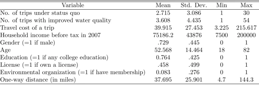
Table 1 shows the summary statistics for our data set. The visitors indicated that
they would on average increase trips by 33%, from 2.7 trips on average to 3.6, if the water
quality were improved. There is large variation in the estimated travel cost per trip, as
the state beach is popular to a large region of Ohio that has limited access to beaches.
The travel cost per trip is estimated as$0.25 per mile multiplied by round-trip miles plus
one-third the respondent’s average wage rate, where their average wage rate is calculated
as their income divided by 2,000.
Other demographic data we collected include the respondent’s gender (73% male), age
(average 52.5 years old), education (76% some college or more), if they have a hunting
or fishing license (46%), or if they are members of an environmental organization (8%).
Similar to Misra et al. (1991), Andrews (2001), Thompson et al. (2002), and Corrigan
et al. (2008), our sample is more male, has higher income, is more educated, and is
older than the general population. We will conclude the paper discussing how our WTP
estimates from the semiparametric smooth coefficient Poisson estimator could be more
easily adjusted for differences between sample and population characteristics, since they
are explicitly a function of the respondent’s demographic variables.
Table 1
here. Table 1
here.
3
Methodology
3.1 Model
Following the basic setup of a mixed Poisson model in Egan and Herriges (2006), we
assume thatyk, the number of trips taken under scenariok, follows a Poisson distribution,
and thatykis associated with unobserved factor (or factors) specific to scenariok, denoted
by vk =exp(uk). The conditional mean of trip counts under scenario k is then assumed
to be an exponential function of covariates and parameters,
E(yk|x, vk) = exp(x
′
β+uk) (1)
wherexis a vector of explanatory variables that are linearly independent by assumption.
This is a fully parametric approach that completely specifies the distribution of the data,
i.e. the outcome variable (trip counts) are assumed to follow a Poisson distribution,
and the conditional mean of trip counts is parameterized to a strict log-linear function.
This linearity assumption of conditional mean, however, may be frequently violated as a
result of nonlinearity or heterogeneity (Winkelmann, 2000), and the violation may not
be easily detected (McLeod, 2011). Moreover, heterogeneous effects are often important
aspects in empirical studies, for instance under the context of this study, we would like to
investigate the heterogeneous welfare impact of improving water quality, but the restrictive
assumptions in the basic mixed Poisson model severely limit its ability to accommodate
these effects (Fr¨olich, 2006).
Some other studies use count data models that relax the common assumption that
the conditional mean function is log-linear. Among those, some have explored
semipara-metric or nonparasemipara-metric approaches, such as Cooper (2000), Jaime and Tudela (2011),
Bach et al. (2017) and Gurmu et al. (1999). Landry and Liu(2009) use a
semiparamet-ric discrete factor method to jointly estimate revealed and stated preference recreation
demand models. Another example is the partially linear model proposed in Robinson
(1988), which has also been used to specify the conditional mean (Cameron & Trivedi,
2003). An overview of methods that allow for various conditional mean assumptions can
be found in Winkelmann (2000) and Cameron and Trivedi (2013).
Although literature in studying the distributional assumption of count data
mod-els exists, we will focus on relaxing the conditional mean specification, and explore a
semiparametric variation of the basic mixed Poisson model. We relax the strict linear
as-sumption on covariatesxby allowing all parameters to vary with a series of demographic
variablesz . The conditional mean of trip counts at scenariok under this semiparametric
assumption is
E(yk|x,z, vk) =exp(x
′
βk(z)+uk) (2)
wherez is a vector of demographic variables that are different from covariatesx. In other
of variables in z, although the exact functional form of βk(·) is left unspecified. Under
the i.i.d. framework, the above semiparametric mixed Poisson model is extended to the regression case after taking the natural logarithm:
lnλik =x
′
iβik(zi) +uik (3)
where λik is the conditional mean trip counts for individuali under scenariok, anduik is
the i.i.d.error that is individual and scenario specific.
Two scenarios are being considered: expected trips under current water quality (k= 1)
and expected trips contingent on water quality being improved (k = 2). Variables in x
include respondent’s travel cost to visit Maumee Bay State Park,Pi, and respondent’s
in-come,Inci, as well as a vector of ones. Vectorzcontains variables indicating respondent’s
demographics, such as gender, age, possession of a hunting or fishing license,
environmen-tal organization membership, and whether the respondent has some college education. A
detailed empirical specification is given by
lnλik =β0ik(zi) +β1ik(zi)Pi+β2ik(zi)Inci+uik. (4)
The specification of this model is essentially the semiparametric smooth coefficient
Poisson model proposed by Li et al. (2002). This model gained popularity for its
distinc-tive flexibility, and has been used in various empirical studies to address heterogeneity
(e.g. Liu,2014,2015). There are obvious benefits of applying this semiparametric mixed
Poisson model to trip responses. The parametersβik(·) are allowed to be unknown smooth
functions, which makes the specification a general case that nicely nests the basic linear
function and other polynomial relationships. Data driven estimation method can obtain
consistent estimates of trip response and parameter values without knowing the functional
form of βik(·).
The most appealing advantage of this semiparametric model lies in its high degree of
flexibility. In a basic log-linear Poisson model the respondent’s demographics enters the
regression function as linear covariates. The coefficient estimates on those demographic
unlikely to hold in practice, because the impact of demographics may well be more than an
intercept shift and can be entangled with income effect and cost responses. For example,
an environmentally conscientious individual may not only take more trips than average,
but also be less sensitive to changes in travel cost and income. The semiparametric
specification can overcome this shortcoming by allowing travel cost and income parameters
to be functions of respondents’ demographics. Demographic variables can directly affect
the number of trips taken under scenario k through the intercept β0ik(·), meanwhile the
impact also indirectly takes place by affecting how trip counts respond to changes in travel
cost and income, i.e. β1ik(·) andβ2ik(·). This flexible specification will produce individual
and scenario specific estimates for all parameters. One of the objectives of this study
is to estimate the consumers’ WTP for improving the water quality. Existing studies
often report a mean estimate of the WTP, and overlook any potential heterogeneity.
With observation specific estimates, we are able to examine whether WTP varies across
visitors, and potentially identify the sources of such heterogeneity.
3.2 Estimation
We estimate the coefficients in equation (4) using the semiparametric smooth coefficient
model following the previous literature of Li et al. (2002), Li and Racine (2010), and Li
et al. (2013). In each paper, an asymptotically consistent estimator is proposed for this
model, while the difference lies in the ability of smoothing discrete variables. The general
idea of these estimators is to apply a kernel smoothing method to fit each observation with
a parametric model (local-constant or local-linear) using a sample of data points close to
the point of interest, i.e. the local sample. The fit largely depends on two key factors: the
smoothing parameter, i.e. the bandwidth, and the kernel function. The bandwidth
deter-mines the size of the local sample, whereas the kernel function, here the Gaussian Kernel,
determines the weight assigned to each data point within the local sample. For instance,
the number of trips taken by individual iis estimated with respondents who have similar
characteristics with individual i. The number of similar respondents considered depends
on the size of the bandwidth, and the weight placed on each respondent when estimating
observations are then smoothed out to obtain a global nonparametric coefficient function.
Given that vector z contains discrete variables only, we will use the estimator proposed
byLi et al.(2013) which is capable of smoothing discrete variables nonparametrically and
removing irrelevant regressors. A detailed description of this estimator is provided in Li
et al. (2013).
The bandwidth or the smoothing parameter plays an important role in the performance
of nonparametric and semiparametric estimation. If the bandwidth is too small, the
coefficient function will be under-smoothed, and the curve will be wiggly; whereas if
the bandwidth is too large, the coefficient function can be over-smoothed and fail to
capture important variations. While Silverman’s rule-of-thumb bandwidth is easy to
compute,2 a data-driven bandwidth selection method is much preferred given that the
density distributions of the coefficients are unknown. This study will use a fully automatic
and data driven method, the least-squares cross-validation (LSCV) method, to select the
bandwidths. This method is based on the principle of minimizing the integrated mean
squared errors of the resulting coefficient estimates (Racine,2008). One advantage of the
LSCV method is that when combined with local-linear fitting, it can automatically detect
the linearity of a coefficient. If a small bandwidth is selected for any z variable in the
coefficient functions, then there is a nonlinear relationship between the variable and the
coefficient (Li & Racine,2007). Hall et al.(2007) suggest that a bandwidth less than one
is considered sufficiently small for a discrete variable, and less than twice the standard
deviation for a continuous variable.
The travel demand under current water quality (scenario k = 1) and hypothetically
improved water quality (scenariok= 2) is estimated with model (4) separately. However,
we return to this in section 5 where we explore joint estimation of the semiparametric
smooth coefficient Poisson model to account for the potential correlation of the two trip
observations from the same respondent. The bandwidths selected for the demographic
variables in each regression are all less than unity, indicating that these variables ought
2
Silverman(1986) derives the optimal choice of bandwidth
h= (4ˆσ
5
3n)
1 5
≈1.06ˆσn
1
5,
to enter the coefficient functions non-linearly and that any attempts to enforce a linear
functional form will result in misspecification and potentially biased WTP estimates.
In the case of over or under dispersion which is common for count data, the
semipara-metric estimator remains consistent, much like the standard Poisson estimator. However,
given the slight overdispersion shown in our data, robust estimation is necessary for valid
statistical inferences. To obtain robust standard errors of all coefficient estimates, we rely
on a residual-based wild bootstrap method which provides asymptotic refinement
with-out imposing the assumption of homoscedasticity (Cameron & Trivedi, 2005).3 Horowitz
(1997, 2001) demonstrates with simulations that the wild bootstrap works better than
other bootstrap methods in the presence of heteroskedasticity.
4
Results
4.1 Coefficient Estimates
The estimation process produces observation specific estimates for both of the scenarios.4
In other words, due to the differences in demographics among visitors, the nonparametric
estimation of coefficient functions is able to fit each visitor with a unique travel demand
estimate and a unique set of coefficient estimates under each water quality scenario. The
coefficients on travel cost is of particular interest, because they are key parameters in the
derivation of the price elasticity of travel demand and consumer surplus. We use the 45°
plot (Henderson et al., 2012) to present these coefficient estimates and their statistical
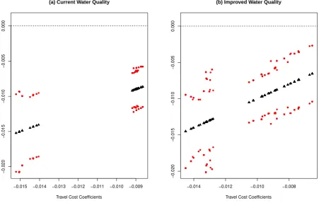
inferences. Figure1shows the estimated coefficients onP (i.e travel cost) along with their
95% confidence intervals for all visitors from the current water quality regression and the
improved water quality regression. The triangles in the plots indicate the coefficient
estimates, and the red dots above and below each estimate are the confidence upper and
lower bounds calculated from bootstrapped standard errors. If the horizontal line at zero
runs outside the confidence interval, then the travel cost coefficient estimate of a particular
3
We first generate bootstrap erroru∗
i based on the regression residual via Mammen’s two-point distribution. We then generate the bootstrap dependent variabley∗
i by adding the bootstrapped error to the fitted value from the regression, i.e. y∗
i =xiˆβ(zi) +u∗i. The bootstrap dependent variableyi∗along with all other covariates are combined into a “bootstrap sample” which is used to estimate bootstrap coefficientβ∗
j. This process is repeated for a large number of times, 4,000, and the standard deviation of all the bootstrap estimates of coefficientβjis calculated as the standard error. The large number of draws was needed to insure convergence.
4
All the analysis in this paper is performed inR. The commands for estimation and testing are available in the ‘np’
observation is significant at the 5% level.
Looking carefully at Figure 1, it shows every individual estimate of the travel cost
coefficient for all the 424 respondents in both scenarios is statistically significant at the
5% level. In addition, these plots also convey the following useful information. First,
the range of the estimates reveals substantial heterogeneity across visitors and between
the two scenarios. Note that the observations in both plots cluster into two groups with
significantly different coefficient estimates. This is driven by demographic characteristics
of visitors, e.g. the education status. In particular, visitors that have been exposed
to some college education are estimated to have smaller travel coefficients (in absolute
value) under both water quality scenarios, and their WTP are likely to be less responsive
to changes in travel cost. Secondly, the travel cost coefficient ranges from -0.015 to -0.008
under the current water quality, and from -0.0145 to -0.006 under the improved water
quality. The minor shift implies that travelers will become slightly less responsive to
travel cost if the water quality at the beach is improved, but the magnitude of change can
be very different across individuals with some individuals having double the estimated
travel cost coefficient versus others. In the appendix, Table 8, we provide the mean
coefficient estimates.
Figure 1
here. Figure 1
here.
4.2 Price Elasticity of Travel Demand
The estimated travel cost coefficients are then used to calculate the price elasticity of
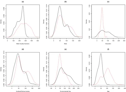
travel demand, which is also individual specific. Panel (a) in Figure2presents the density
distributions of travel demand price elasticity, where the solid black line is for the expected
travel demand under current water quality and the dashed red line is for the expected
travel demand contingent on water quality being improved. The information revealed by
these distributions are consistent with the previous discussion. The travel cost demand
elasticity, i.e. how sensitive travelers are to changes in travel cost, varies substantially,
ranging from -1.883 to -0.031 with a mean of -0.404 under the current scenario, and from
-1.791 to -0.032 with a mean of -0.388 under the improved scenario.
−0.015 −0.014 −0.013 −0.012 −0.011 −0.010 −0.009
−0.020
−0.015
−0.010
−0.005
0.000
(a) Current Water Quality
Travel Cost Coefficients
−0.014 −0.012 −0.010 −0.008
−0.020
−0.015
−0.010
−0.005
0.000
(b) Improved Water Quality
[image:13.595.86.538.252.539.2]Travel Cost Coefficients
Figure 1: Observation Specific Travel Cost Coefficients
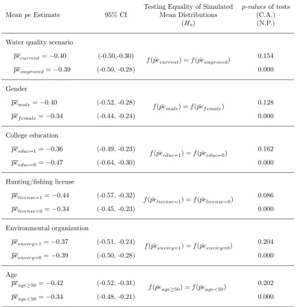
elasticity estimates before and after improving the water quality. Firstly, in Table 2, row
2, as is routine, we report the 95% confidence interval (C.I.) for our price elasticity point
estimates. The confidence intervals largely overlap. However, Poe et al. (1994) and Poe
et al.(2005) clearly demonstrate that it is incorrect to use the nonoverlapping confidence
interval because the significance level is overstated.
Therefore, we turn to statistical distribution tests to determine if the distributions
of mean price elasticity under the two scenarios are significantly different. We first use
the wild bootstrap method to produce a simulated distribution of the mean price
elas-ticity under each scenario. We then use the convolutions approach (C.A.) of measuring
simulated distributions proposed in Poe et al. (1994) and Poe et al. (2005)5, and the
nonparametric equality of densities test (N.P.) developed by Li et al. (2009) to compare
the distributions of mean price elasticity estimates before and after improving the water
quality.6 Considering the distributions are unknown, we opt for these two nonparametric
tests. The test results are also reported in the second row of Table 2. The null
hypoth-esis of the test is the equality of the two distributions. The p value of the convolutions
approach is 0.154 and thus the null hypothesis cannot be rejected. However, the p value
of the nonparametric equality of densities test is 0 leading to the rejection of the null
hypothesis, which implies a location shift from one distribution to the other. This test
result suggests that travel demand is expected to become slightly less elastic to changes
in travel cost if the water quality at the beach is improved. However, looking again at
Figure 2 panel (a), the difference in the distributions appears small, and lends support
to the results from the convolution’s approach. For the remainder of the paper we report
the results from both tests, and we leave it to future research to explore further their
implications. Figure 2
here. Figure 2
here.
4.3 Heterogeneous Price Elasticity
Since the travel cost coefficients, hence the price elasticities, are jointly determined by
all demographic variables included in the coefficient function, it is difficult to completely
5
To achieve stable results a large number of simulations is needed; we used 4000 draws.
6
−2.0 −1.5 −1.0 −0.5 0.0 0.0 0.5 1.0 1.5 2.0 (a)
Water Quality Scenario
Density
−1.5 −1.0 −0.5 0.0
0.0 0.5 1.0 1.5 2.0 (b) Male Density
−1.5 −1.0 −0.5 0.0
0.0 0.5 1.0 1.5 2.0 2.5 (c) Education Density
−1.5 −1.0 −0.5 0.0
0.0 0.5 1.0 1.5 2.0 2.5 (d) Hunting/Fishing License Density
−1.0 −0.5 0.0
0.0 0.5 1.0 1.5 2.0 (e) Environmental Org. Density
−1.5 −1.0 −0.5 0.0
[image:15.595.78.510.164.489.2]0.0 0.5 1.0 1.5 2.0 2.5 (f) Age Density
Figure 2: Distribution of Estimated Price Elasticity of Travel Demand by Scenario and Demographics
Panel (a): Distribution of price elasticity estimates of all visitors under current (solid black line) v.s. improved water quality scenario (dashed red line).
Panel (b): Distribution of price elasticity estimates of male visitors (solid black line) v.s. female visitors (dashed red line) under improved water quality scenario.
Panel (c): Distribution of price elasticity estimates of visitors with college education (solid black line) v.s. visitors without college education (dashed red line) under improved water quality scenario.
Panel (d): Distribution of price elasticity estimates of visitors with hunting or fishing licenses (solid black line) v.s. visitors without hunting or fishing licenses (dashed red line) under improved water quality scenario.
Panel (e): Distribution of price elasticity estimates of visitors who are associated with environmental organizations (solid black line) v.s. visitors who are not associated with any environmental organization (dashed red line) under improved water quality scenario.
disentangle the impact of each demographic variable. Plotting the individual price
elas-ticities by demographic variables, as in Figure2, panels (b) through (f), is one of the most
efficient means for that purpose. The estimates of price elasticities under the improved
scenario are used given that we are more interested in the outcomes of the improved
water quality scenario. For instance in the second panel, panel (b), the distributions are
for female respondents (“Male=0”; dashed red line) and male respondents (“Male=1”;
solid black line). The distribution for females is shifted rightward (price elasticities closer
to zero), suggesting that the majority of female visitors are relatively less responsive to
changes in travel cost than male visitors. Again we use the convolutions approach and the
nonparametric equality of densities test to statistically determine if the simulated mean
price elasticity distributions between male and female visitors are different. As reported
in Table 2, we again find different results from the two nonparametric tests with the
con-volutions approach not rejecting the null hypothesis of equal simulated mean distributions
(p-value of 0.128) and the nonparametric equality of densities test easily rejecting this null
hypothesis (p-value of 0).
Table 2
here. Table 2
here.
Similar analysis applies to the other three binary demographic variables. From panel
(c) in Figure2, we can see that the price elasticities of beach visitors with college education
are smaller in absolute value than those without college education. The equal distribution
test result from the nonparametric equality of densities test, shown in Table 2, implies
that travelers with college education are significantly less sensitive to travel cost. This
result is expected for two reasons. First, individuals who have been exposed to higher
education are likely to care more about the environment, and their demand for travel may
not be affected by travel cost as much as others. The other reason is that, travelers with
college education are more likely to have full time jobs with paid vacations which again
makes them less elastic to travel cost. However, again the convolutions approach, with a
p-value of 0.128, cannot reject the null hypothesis of equal distributions.
The possession of a hunting or fishing license is another source of heterogeneity in
travel cost responsiveness. Panel (d) of Figure 2 and the testing results in Table 2 both
cost than those who do not. Public beach is typically popular among casual visitors, but
may not be the most preferred fishing or hunting spots. If this is taken into consideration,
travelers who prioritize fishing or hunting experience may be more sensitive to travel cost
and easily opt for other alternatives. This demographic characteristic is the only one with
both nonparametric tests rejecting the null hypothesis at the 10% significance level.
Panel (e) in Figure 2 shows a small change in the distribution of the price elasticity
for travelers affiliated with an environmental organization, and again our tests report
different results for the null hypothesis of equal distributions. From the convolution test
we conclude that environmental organization membership makes no significant difference
in travelers’ responsiveness to changes in travel cost, even if we expect those who are a
part of an environmental organization to value environmental amenities more.
There are a total of eight age groups in our sample ranging from age 18 to age 82. We
test the price elasticities across groups, and find that there is not much difference across
four younger age groups, nor within four older age groups. Based on this observation, we
create a binary variable which takes a value of 1 for visitors at or above 50 years old, and 0
otherwise. Among the younger age group (consisting 43% of the sample), 73% of visitors
are at age 40s and 23% of visitors are at age 30s. Therefore, the majority of this group are
middle aged travelers. Panel (f) of Figure2depicts the distributions of price elasticity for
both age groups, and it appears that price elasticity of older visitors is larger in absolute
value than that of younger visitors. Such a finding is reasonable, because compared with
older groups, middle aged travelers are likely to have more time constraints, hence higher
opportunity cost, therefore they are likely to be less responsive to travel cost. However,
again, only the nonparametric equality of densities test rejects the null hypothesis.
Before turning next to WTP estimates, these detailed price elasticity estimates could
be used by resource managers to better forecast changes in visitation if, for example,
gasoline prices or the state gasoline tax changed substantially.7 Particularly, we find a
robust difference in price elasticity estimates for those with a hunting or fishing license
versus those without, and as all the panels in Figure 2 show, there is large variation in
the individual level price elasticity estimates, e.g., some males with inelastic demand and
7
other males with elastic demand (panel (b)).
4.4 Willingness to Pay Estimates
The ultimate goal of this study is to find out respondents’ WTP for improving the water
quality at the Maumee Bay State Park Beach, which can be achieved by calculating the
difference in consumer surplus of travel demand under the two water quality scenarios.
From the specification of travel cost model (4), the mean consumer surplus for individual
i under senario k can be given by
CSik =−
λik
β1ik(zi)
. (5)
Individual i’s WTP and its estimate are
W T Pi =CSi2−CSi1
W T Pi =
λi2 −β1i2(zi)
− λi1
−β1i1(zi)
, (6)
whereλi2 andβ1i2(zi) are the trip counts and travel cost coefficient for individuali
contin-gent on water quality being improved; and λi1 and β1i1(zi) are the trip counts and travel
cost coefficient for individual i under the status quo.
When estimating consumer surplus, whether to use fitted trips or actual trips depends
on the assumptions made as to the source of the error term. If the error is due to
specification error, then actual trips is appropriate to calculate consumer surplus; whereas
if the error comes from measurement errors in trip counts, then fitted trips should be used
(Bockstael & Strand Jr., 1987; Haab & McConnell, 1996). Though both types of errors
are likely to be present in reality, we believe measurement error is the primary source
in our case because the added flexibility of the semiparametric travel demand model can
reduce specification error. Therefore we use fitted trips. Figure 3
here. Figure 3
here.
The individual specific consumer surplus under each water quality scenario is
cal-culated based on equation (5) using the parameter estimates from the two regressions
respectively. The density plots in panel (a) of Figure 3 provide a more comprehensive
0 100 200 300 400 500 0.000 0.002 0.004 0.006 0.008 (a)
Water Quality Scenario
Density
0 50 100 150 200
0.000 0.002 0.004 0.006 0.008 0.010 0.012 0.014 (b) Male Density
0 50 100 150 200 250
0.00 0.01 0.02 0.03 0.04 (c) Education Density
0 50 100 150 200
0.000 0.002 0.004 0.006 0.008 0.010 0.012 0.014 (d) Hunting/Fishing License Density
−50 0 50 100 150 200 250
0.000 0.002 0.004 0.006 0.008 0.010 0.012 0.014 (e) Environmental Org. Density
0 50 100 150 200 250
[image:19.595.74.514.159.480.2]0.000 0.005 0.010 0.015 0.020 (f) Age Density
Figure 3: Distribution of Estimated Consumer Surplus and Willingness to Pay by Scenario and Demo-graphics
Panel (a): Distribution of consumer surplus estimates of all visitors under current (solid black line) v.s. improved water quality scenario (dashed red line).
Panel (b): Distribution of WTP estimates of male visitors (solid black line) v.s. female visitors (dashed red line) under improved water quality scenario.
Panel (c): Distribution of WTP estimates of visitors with college education (solid black line) v.s. visitors without college education (dashed red line) under improved water quality scenario.
Panel (d): Distribution of WTP estimates of visitors with hunting or fishing licenses (solid black line) v.s. visitors without hunting or fishing licenses (dashed red line) under improved water quality scenario.
Panel (e): Distribution of WTP estimates of visitors who are associated with environmental organizations (solid black line) v.s. visitors who are not associated with any environmental organization (dashed red line) under improved water quality scenario.
surplus under current water quality, and the dashed red line is the estimated consumer
surplus contingent on the water quality being improved. The estimated range of consumer
surplus from trip demand under the improved scenario shows a larger variation with a
greater mean and a higher upper bound. To test whether the difference is significant, we
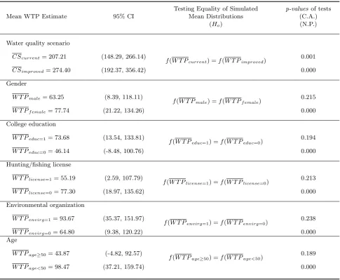
apply the same analysis as for the price elasticity. Both the convolutions test and the
non-parametric equality of densities test, reported in the second row of Table 3, suggest that
the distribution of simulated mean consumer surplus after improving the water quality is
significantly different than that under the status quo. These results imply that improving
water quality increases the overall consumer surplus. Table 3
here. Table 3
here.
The difference between the two consumer surplus estimates for each traveler are then
calculated using equation (6) as an estimate of the traveler’s WTP for improving the
water quality at the beach. The estimates of WTP are plotted in Figure 4 with a mean
of $67.18, the wide range of which suggests that the amount of welfare increase is again
heterogeneous across visitors and having a generally nonparametric shape. Figure 4
[image:20.595.172.416.417.621.2]here. Figure 4
here.
0 50 100 150 200 250
0.000
0.002
0.004
0.006
0.008
0.010
0.012
Estimates of Willingess to Pay for Improvement
Density
Figure 4: Distributions of Estimated Willingness to Pay
Distribution of estimated WTP for improving water quality.
4.5 Heterogeneous Willingness to Pay
To explore the heterogeneity in travelers’ WTP for improved water quality, the estimates
through (f). We can see that WTP estimates vary substantially by the five demographic
variables. The mean WTP estimates of the demographic groups are summarized in Table
3. Discussing the five variables in order of the largest percent change for the mean WTP
estimates, first is age in Panel (f), Figure 3. As in the analysis of heterogeneous price
elasticity, we categorize all visitors into two larger age groups, above or below 50 years
old. Panel (f) shows that younger visitors (“Age=0”, mostly at 30s and 40s) are willing to
pay substantially more than older visitors for the improved water quality (mean WTP of
$98 v.s. $44; a 124% increase). Similarly, in spite of larger variation, travelers with some
college education (panel (c)) show greater WTP for improved water quality than those
without any higher education (mean WTP of $74 v.s. $46; a 60% increase). Those who
are affiliated with an environmental organization (panel (e)) are also willing to pay more
for improved water quality than others (mean WTP of $94 v.s. $65; a 45% increase).
The WTP of visitors who do not have a fishing or hunting license (panel (d)) is generally
higher than those who do have such a license (mean WTP of$77 v.s. $55; a 40% increase).
Again, this is likely because the public beach is not the high worth location for anglers.
Lastly, the least difference is observed comparing female visitors to male visitors with
women estimated to be willing to pay more for the improved water quality than male
visitors (mean WTP of $78 v.s. $63; a 23% increase).
Besides visualizing the WTP distributions and comparing the mean WTP estimates
by demographic groups, it is necessary to formally test if the mean WTP difference
is statistically significant between groups. The testing results are reported in Table 3,
and similar to the price-elasticity heterogeneity analysis, the nonparametric equality of
densities test always has p-values of 0 whereas the convolutions approach has p-values
ranging from 0.19 to 0.22. Thus the nonparametric equality of densities test confirms that
the visually identified difference in WTP by gender, education, etc., are all statistically
significant. However, for the convolutions approach thep-values are too high and thus the
null hypothesis of equal simulated mean WTP distributions cannot be rejected. While
we referenced earlier it is not appropriate to use the nonoverlapping confidence interval
criteria, all the 95% confidence intervals do overlap significantly, suggesting to us the
to investigate further.
Recall in section 4.2 we find that less elastic travel demand is associated with such
characteristics of travelers as being female, middle aged, with some college education, not
owning a fishing or hunting license, and being a member of an environmental organization,
etc. These demographic groups are also those who gain larger amounts of benefits, thus are
willing to pay more for improving the water quality at the beach than their counterparts.
5
Alternative Specifications
5.1 Parametric Specification Alternative
Our results so far have provided estimates for price elasticities, consumer surplus, and
WTP under two water quality scenarios. The findings have also indicated that visitors
respond to changes in travel cost (i.e. price elasticity of travel demand) differently, and
that the welfare gain as a result of improved water quality is heterogeneous across various
demographic groups. Now we turn towards an alternative parametric specification for
comparison.
The equations below formalize the univariate Poisson-lognormal mixture model (UVPLN)
for the trip demand under current water quality (k = 1) and improved water quality
(k = 2).
E(yk|x,z, vk) = exp(x
′
βk+z
′
γk+uk)
lnλik =x
′
iβk+z
′
iγk+uik (7)
where the conditional mean trip counts λik are log-linear functions of travel cost and
income in x and demographic variables in z. βk and γk are constant parameters to
be estimated for each scenario separately. This model, like the semiparametric smooth
coefficient estimator, begins with the basic Poisson count data model. One difference is
that the Poisson-lognormal mixture model is fully parametric, mixing a lognormal error,
expuk, that accounts for unobserved heterogeneity. As Landry and Liu (2009) discuss,
asymptotically efficient. However, the estimates could be biased and inconsistent if the
normality assumption is not met. In contrast, the semiparametric smooth coefficient
estimator is an asymptotically consistent estimator without specifying any functional
form for the unobserved heterogeneity. Moreover, similar to a latent class model, the
unobserved heterogeneity is captured via slope coefficients for the explanatory variables
(Hynes & Greene, 2013), but with the semiparametric smooth coefficient estimator, no
arbitrary number of latent classes needs to be determined.
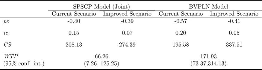
The estimates of elasticities, consumer surplus and WTP from this specification are
reported in the “UPLN Model” segment of Table4.8 A direct comparison with the results
from the semiparametric model would be difficult since all the estimates are individual
specific. Nonetheless, we calculate the mean estimates of all parameters, and summarize
them in the “SPSC Model” segment of Table4. Firstly, as in the semiparametric
specifi-cation, contingent trips assuming improved water quality are less responsive to travel cost
(i.e., the price elasticity of demand decreases in absolute value). This finding is similar
to Whitehead et al. (2008) and Awondo et al. (2011). The mean WTP estimate from
the UVPLN model is substantially higher at$164 versus the$67 from the semiparametric
model. Given that we found statistically significant individual level travel cost coefficients
for all 424 respondents (Figure 1), the clear nonparametric distributions we find for the
estimated consumer surplus distributions (Figure 4, panel (a)), and the estimated WTP
distribution (Figure 3), we conclude the semiparametric smooth coefficient estimator fits
our data better, and the resulting lower WTP estimate is more accurate.
We also investigated both models’ sensitivity to outliers. In the data section we noted
that six observations were dropped, and in footnote 1 we stated that the semiparametric
model mean WTP estimate increases 18% when these six observations were instead
in-cluded. In contrast, with the UVPLN model, with the six observations added, the mean
WTP estimate decreases 63% from $163.8 to $61.3. The outliers are high trip count and
low travel cost observations. As noted in the data section, many recreation demand
stud-ies drop these observations to ensure the modeling of visitors instead of nearby locals.
However, there can be uncertainty on which trip observations are too high with too low
8
a price. All else equal, we prefer an estimation method that minimizes the impact of this
decision. Therefore, we see another advantage of the semiparametric model is that it does
a better job in retaining impact locally rather than averaging over the entire sample. For
the semiparametric model, the individual WTP estimates only increase for the few
obser-vations near the outliers. Whereas for the UVPLN model the price elasticities increase
substantially in absolute value (from around -0.5 to -0.9) showing the outliers are causing
the whole estimated recreation demand curve to be more elastic and thus a lower mean
WTP estimate. This finding is consistent with Landry and Liu(2009) who also note that
the Poisson-lognormal model is sensitive to outliers.
5.2 Joint Estimation of the Two Scenarios
A limitation of our analysis so far is ignoring the pseudo-panel nature of our data, where
each respondent provides their observed trips given current water quality and their
con-tingent trips given the proposed improved water quality scenario. As an alternative
spec-ification, we pool the data from both scenarios and allow the coefficients to vary across
the two scenarios by adding a binary variable “current scenario” to the vectorz. We then
cluster the standard errors to account for the within-person correlation. One difficulty
with the smooth coefficient estimator is that pooling the data affects the bandwidths
se-lection of allz variables (see equation 4). In particular, pooling the data leads to the same
person being used as their own neighbor in the local fit of the coefficients. Our solution
is to set the bandwidth of “current scenario” to zero, and use the original bandwidths
for all the z variables from the “improved scenario” estimation. Then we estimate this
pooled data model using clustered standard errors. We reproduce many of the previous
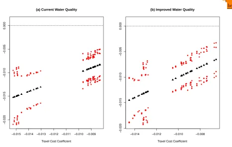
tables and figures for comparison. Figure 5 shows again the estimated coefficients on P
(i.e. travel cost) and their 95% confidence intervals for all visitors from the one pooled
data regression. Comparing to Figure 1, the results are unchanged in that all individual
price coefficients being statistically significant for both water quality scenarios. In the
ap-pendix, Table 9, we show the mean coefficient point estimates from the joint estimation.
Comparing to Table8, the coefficients only change by a small amount. Next in Table5we
as the consumer surplus and WTP estimates from the joint estimation. Comparing to
Table 4, given the price coefficient individual estimates change little, we also see that the
mean elasticity estimates are unchanged and the consumer surplus and WTP estimates
only change by a small amount (less than one dollar). With clustered standard errors
[image:25.595.81.548.203.499.2]from the pooled data, the 95% confidence interval for the WTP estimate widens slightly.
Figure 5
here. Figure 5
here.
−0.015 −0.014 −0.013 −0.012 −0.011 −0.010 −0.009
−0.020
−0.015
−0.010
−0.005
0.000
(a) Current Water Quality
Travel Cost Coefficient
−0.014 −0.012 −0.010 −0.008
−0.020
−0.015
−0.010
−0.005
0.000
(b) Improved Water Quality
Travel Cost Coefficient
Figure 5: Observation Specific Travel Cost Coefficients (Joint Estimation of Two Scenarios)
The semiparametric coefficients on travel cost for each beach visitor from jointly estimating trip demand under the two water quality scenarios are presented. Standard errors are clustered by visitor. The dots above and below each estimate are the bootstrapped 95% confidence upper and lower bounds.
For comparison, we also updated our Poisson-lognormal paramateric estimates, now
using a bivariate Poisson-lognormal model (BVPLN) following Awondo et al.(2011)
simi-lar to their MVPLN1 specification. This restricted form mimics the multivariate
Poisson-gamma mixture model (MPG) that is based on Winkelmann (2000)’s nomenclature,
ex-cept that instead of a univariate gamma error, a univariate lognormal error is utilized
(Awondo et al.,2011). Also, to match the separate UVPLN regressions we currently have
in Table 4, we allow coefficients on all the variables - price, income, gender, age,
educa-tion, license, and environmental organization - to vary between the two scenarios.9 Our
9
BVPLN is exactly the same as if we pooled the UVPLN data and ran clustered standard
errors, as the BVPLN allows for all the same coefficients as before, except now there
is a common error term at the individual level. Again, comparing Table 4 to Table 5,
we see the price elasticity estimates change slightly, the income elasticities are the same,
the consumer surplus estimates increase at most 5.7% (for the improved scenario) and
thus the WTP estimate increases 5%. Finally, in contrast to the semiparametric smooth
coefficient estimator, we find that the WTP 95% confidence interval narrows.
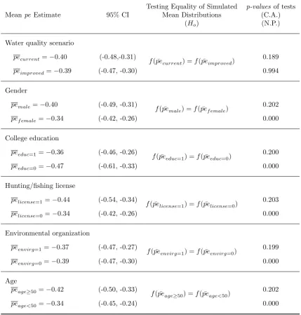
Table6reproduces the price elasticity estimates. Comparing to Table2the mean price
elasticity point estimates are all the same, but the 95% confidence intervals and p-values
for the two nonparametric tests are slightly different. For the convolutions approach the
p-values are mostly a little higher, and the p-values from the nonparametric equality of
densities test are the same at 0. The only exception for the nonparametric equality of
densities test is a large increase in the p-value testing the equality of simulated mean
price elasticity from the two water quality scenarios, where now the null hypothesis of
equality is not rejected. Similarly, Table 7 compared to Table 3 shows small changes in
the mean WTP estimates and the 95% confidence intervals. Turning to the p-values for
the nonparametric tests, the p-values for the nonparametric equality of densities test are
again the same or slightly higher, whereas for the convolutions approach thep-values are
all slightly lower except for age whose p-value is significantly lower. Now with ap-value of
0.075, we can reject the null hypothesis of equal simulated mean WTP distributions, and
conclude those under the age of 50 have statistically significantly higher mean WTP at
the 10% level. This is similar to the latent-class approach finding a class of respondents
that has significantly different WTP estimates than others.
Poe et al. (1997) find similar results to ours with their estimation of contingent
valu-ation data where the survey respondents provided two binary responses. They conclude
their estimation of joint models has a small effect on the distributions of estimated mean
WTP. However, similarly they find that accounting for the correlation does impact the
hy-pothesis that the mean WTP is significantly different across scenarios with their p-values
decreasing once the correlation is included. With the convolutions approach we also find
that cross-equation equality restrictions reduce the standard errors of their coefficients.
We have not imposed any cross-equation equality restrictions. For example, we could
impose the restriction that the coefficients for the gender dummy variable must be equal
for the two water quality scenarios. We have instead mimicked the separate regressions
with none of these restrictions, and observed how the results changed when we only pooled
the data and used clustered standard errors. We continue to find mixed results where
the nonparametric equality of densities test shows statistically significantly different price
elasticities and mean WTP estimates across our five included demographic variables.
Whereas the convolutions approach finds only a statistically significant difference for
the price elasticities for those with a hunting/fishing license and analyzing the scenarios
separately (see Table2), and also for the mean WTP estimates for the respondents younger
than 50 and analyzing the scenarios jointly (see Table7). We leave it to future research to
explore further the application of these two nonparametric tests and also the importance
of cross-equation equality restrictions when doing joint estimation. Table 4
here. Table 4
here.
6
Conclusion
We introduced a semiparametric smooth coefficient Poisson model to a count data
recre-ation demand framework and showed the rich and flexible heterogeneity that can be
included with such an approach. We show that our sample of visitors each has an
indi-vidual statistically significant price coefficient estimate leading to clearly nonparametric
consumer surplus and willing to pay distributions. We compare the WTP estimates from
the semiparametric smooth coefficient Poisson model to a fully parametric alternative,
the Poisson-lognormal mixture model, and we find substantially different WTP estimates
and we conclude the lower WTP estimates from the semiparametric smooth coefficient
estimator are more accurate for our data. We also show that our WTP estimates vary
based on every demographic variable we have for our sample of beach visitors with all
of our results consistent with economic theory. With our approach, we show how the
WTP estimates vary for each demographic variable, without resorting to constraining the
visitors to a small number of classes as the previous literature has done using the latent
differences in price elasticity estimates and WTP estimates. Using a joint estimation with
cross equation restrictions may be important to limit the number of coefficients estimated
in a meaningful way to increase the statistical significance of the results, similar to a
latent class analysis limiting the number of included classes.
In general, this flexibility is valuable for future researchers who can include any
vari-ables of interest beyond the standard demographic varivari-ables we have included here. And
the richer results, price elasticities, consumer surplus and WTP estimates, are valuable to
planners and policymakers who can easily see how all these estimates vary with
charac-teristics of the population of interest. If demographics change over time, our richer results
can be used to show how WTP estimates will change.
For our water quality improvement scenario we find a mean visitor annual WTP of
approximately $67. However, returning to the issue that our sample of visitors is more
male, older, more educated, and higher income than the general population of visitors, if
we knew the basic demographics of the population of visitors to our site of interest than we
could adjust all of our demographic specific WTP estimates, including the overall mean
WTP. Unfortunately, we do not have that information for our site of interest. Moreover,
as Creel and Loomis (1997) point out, we could also use our enriched WTP estimates
in a more advanced benefit transfer to a similar project somewhere else, converting from
local demographics to the different demographics elsewhere. Lastly, our conditional WTP
estimates allow us to explore distributional issues. For example, we find that less
edu-cated visitors have lower estimated WTP for the water quality improvement. Our WTP
estimates would be convenient as benefit estimates in a distributionally weighted
benefit-cost analysis (Boardman et al., 2017). Also, for example, if the resource managers at the
beach were considering the distributional impacts of a user fee, they could use our price
elasticities to see who are likely to change their behavior and reduce trips, and also how
that would impact the overall and WTP estimates, conditional on any of the demographic
variables we have included.
In conclusion, our intuitive and insightful results show the power of modeling
respon-dent heterogeneity with a semiparametric smooth coefficient Poisson method. We show
sce-narios separately or jointly, which is also true for the fully parametric Poisson-lognormal
method. Instead, the major difference in WTP estimates is moving from the fully
para-metric model to our semiparapara-metric method that allows for heterogeneity of preferences
in a more flexible way. In many instances researchers and policymakers are interested in
how the WTP estimates vary within the population of interest. Usually a latent class type
model is most popular which limits the analysis to a few classes. We think if researchers
are considering a latent class framework, then our semiparametric smooth coefficient
es-timator should be considered. In this paper, we provide all the necessary statistical
methods for finding statistically and economically significantly different price elasticities,
consumer surplus, and WTP estimates for any included demographic variable, discrete,
or continuous. Finally, future research could expand our analysis to include nonusers.
Appendix
This appendix provides the summary of coefficient estimates from the semiparametric
smooth coefficient mixed Poisson model when the two scenarios are estimated separately
References
Allenby, G. M., Arora, N., & Ginter, J. L. (1998). On the Heterogeneity of Demand.Journal of Marketing
Research,35(3), 384-389. doi: 10.2307/3152035
Allenby, G. M., & Rossi, P. E. (1999). Marketing Models of Consumer Heterogeneity. Journal of
Econometrics,89(1-2), 57-78. doi: 10.1016/S0304-4076(98)00055-4
Andrews, T. (2001, 01). A Contingent Valuation Survey of Improved Water Quality in the Brandywine
River: An Example of Applied Economics in the Classroom. Pennsylvania Economic Review,
10, 1-13.
Awondo, S. N., Egan, K. J., & Dwyer, D. F. (2011). Increasing Beach Recreation Benefits by Using
Wetlands to Reduce Contamination. Marine Resource Economics, 26(1), 1-15. doi: 10.5950/
0738-1360-26.1.1
Bach, P., Farbmacher, H., & Spindle, M. (2017). Semiparametric Count Data Modeling with an
Appli-cation to Health Service Demand. Econometrics and Statistics. doi: https://doi.org/10.1016/
j.ecosta.2017.08.004
Baerenklau, K. A. (2010). A Latent Class Approach to Modeling Endogenous Spatial Sorting in Zonal
Recreation Demand Models. Land Economics,86(4), 800816. doi: 10.3368/le.86.4.800
Boardman, A., Greenberg, D., Vining, A., & Weimer, D. (2017). Cost-Benefit Analysis: Concepts and
Practice(4th ed.). Cambridge University Press.
Bockstael, N. E., & Strand Jr., I. E. (1987). The Effect of Common Sources of Regression Error on
Benefit Estimates. Land Economics, 63(1), 11-20. doi: 10.2307/3146652
Boxall, P., & Adamowicz, W. (2002). Understanding Heterogeneous Preferences in Random Utility
Models: A Latent Class Approach. Environmental and Resource Economics, 23(4), 421-442.
doi: 10.1023/A:1021351721619
Bujosa, A., Riera, A., & Hicks, R. L. (2010). Combining Discrete and Continuous Representations of
Preference Heterogeneity: A Latent Class Approach. Environmental and Resource Economics,
47(4), 477493. doi: 10.1007/s10640-010-9389-y
Cameron, A. C., & Trivedi, P. K. (2003). Essentials of Count Data Regression. In B. H. Baltagi
(Ed.),A Companion to Theoretical Econometrics (p. 331-348). Blackwell Publishing Ltd. doi:
10.1002/9780470996249.ch16
Cameron, A. C., & Trivedi, P. K. (2005). Microeconometrics: Methods and Applications. Cambridge,
UK: Cambridge University Press.
Cameron, A. C., & Trivedi, P. K. (2013). Regression Analysis of Count Data. Cambridge: Cambridge
University Press.
Cooper, J. (2000, 05). Nonparametric and Semi-Nonparametric Recreational Demand Analysis.American
Corrigan, J. R., Kling, C. L., & Zhao, J. (2008). Willingness to Pay and the Cost of Commitment: An
Empirical Specification and Test.Environmental and Resource Economics,40(2), 285-298. doi:
10.1007/s10640-007-9153-0
Creel, M., & Loomis, J. (1997). Semi-nonparametric Distribution-Free Dichotomous Choice Contingent
Valuation. Journal of Environmental Economics and Management, 32(3), 341 - 358. doi:
https://doi.org/10.1006/jeem.1997.0972
Dillman, D. (2007). Mail and Internet Surveys, the Tailored Design Method (2nd ed.). John Wiley and
Sons, Inc.
Egan, K., Corrigan, J. R., & Dwyer, D. F. (2015). Three Reasons to Use Annual Payments in Contingent
Valuation Surveys: Convergent Validity, Discount Rates, and Mental Accounting. Journal of
Environmental Economics and Management,72, 123-136. doi: 10.1016/j.jeem.2015.05.002
Egan, K., & Herriges, J. (2006). Multivariate Count Data Regression Models with Individual Panel
Data from an On-site Sample. Journal of Environmental Economics and Management, 52(2),
567-581. doi: 10.5950/0738-1360-26.1.1
Englin, J., & Shonkwiler, J. S. (1995). Modeling Recreation Demand in the Presence of
Unobserv-able Travel Costs: Toward a Travel Price Model. Journal of Environmental Economics and
Management,29(3), 368-377. doi: 10.1006/jeem.1995.1053
Fr¨olich, M. F. (2006). Non-parametric Regression for Binary Dependent Variables. The Econometrics
Journal,9(3), 511-540. doi: 10.1111/j.1368-423X.2006.00196.x
Gurmu, S., Rilstone, P., & Stern, S. (1999). Semiparametric Estimation of Count Regression Models.
Journal of Econometrics,88(1), 123-150. doi: https://doi.org/10.1016/S0304-4076(98)00026-8
Haab, T. C., & McConnell, K. E. (1996). Count Data Models and the Problem of Zeros in Recreation
Demand Analysis. American Journal of Agricultural Economics, 78(1), 89-102. doi: 10.2307/
1243781
Hall, P., Li, Q., & Racine, J. S. (2007). Nonparametric Estimation of Regression Functions in the
Presence of Irrelevant Regressors.The Review of Economics and Statistics,89(4), 784-789. doi:
10.1162/rest.89.4.784
Henderson, D. J., Kumbhakar, S. C., & Parmeter, C. F. (2012). A Simple Method to Visualize Results
in Nonlinear Regression Models. Economics Letters, 117(3), 578-581. doi: https://doi.org/
10.1016/j.econlet.2012.07.040
Horowitz, J. L. (1997). Bootstrap Methods in Econometrics: Theory and Numerical Performance. In
D. M. Kreps & K. F. Wallis (Eds.), Advances in economics and econometrics: Theory and
applications: Seventh world congress (Vol. 3, p. 188222). Cambridge University Press. doi:
10.1017/CBO9781139051996.007
Elsevier. doi: https://doi.org/10.1016/S1573-4412(01)05005-X
Hynes, S., & Greene, W. (2013). A Panel Travel Cost Model Accounting for Endogenous Stratification
and Truncation: A Latent Class Approach. Land Economics, 89(1), 177-192. doi: 10.3368/
le.89.1.177
Jaime, M. M., & Tudela, A. M. (2011). Valuing a Water Recreation Facility Using Semi Parametric
Estimators in the Travel Cost Method. Cuadernos de Econom´ıa,30, 217 - 233.
Landry, C. E., & Liu, H. (2009). A Semi-parametric Estimator for Revealed and Stated Preference Data
- An Application to Recreational Beach Visitation. Journal of Environmental Economics and
Management,57(2), 205-218. doi: 10.1016/j.jeem.2008.05.002
Li, Q., Huang, C. J., Li, D., & Fu, T.-T. (2002). Semiparametric Smooth Coefficient Models. Journal of
Business and Economic Statistics,20(3), 412-422. doi: 10.1198/073500102288618531
Li, Q., Maasoumi, E., & Racine, J. S. (2009). A Nonparametric Test for Equality of Distributions with
Mixed Categorical and Continuous Data. Journal of Econometrics, 148(2), 186 - 200. doi:
https://doi.org/10.1016/j.jeconom.2008.10.007
Li, Q., Ouyang, D., & Racine, J. S. (2013). Categorical Semiparametric Varying-Coefficient Models.
Journal of Applied Econometrics,28(4), 551-579. doi: 10.1002/jae.1261
Li, Q., & Racine, J. S. (2007). Nonparametric Econometrics: Theory and Practice. Princeton: Princeton
University Press.
Li, Q., & Racine, J. S. (2010). Smooth Varying-Coefficient Estimation and Inference for Qualitative and
Quantitative Data.Econometric Theory,26(06), 1607-1637. doi: 10.1017/S0266466609990739
Liu, W. (2014). Modeling Gasoline Demand in the United States: A Flexible Semiparametric Approach.
Energy Economics,45, 244 - 253. doi: 10.1016/j.eneco.2014.07.004
Liu, W. (2015). Gasoline Taxes or Efficiency Standards? A Heterogeneous Household Demand Analysis.
Energy Policy,80, 54 - 64. doi: 10.1016/j.enpol.2015.01.029
McLeod, L. (2011). A Nonparametric vs. Latent Class Model of General Practitioner Utilization:
Ev-idence from Canada. Journal of Health Economics, 30(6), 1261 - 1279. doi: https://doi.org/
10.1016/j.jhealeco.2011.08.005
Misra, S. K., Huang, C. L., & Ott, S. L. (1991). Consumer Willingness to Pay for Pesticide-Free Fresh
Produce. Western Journal of Agricultural Economics,16(2), 218 - 227.
Morey, E., Thacher, J., & Breffle, W. (2006). Using Angler Characteristics and Attitudinal Data to
In-dentify Environmental Preference Classes: A Latent-Class Model. Environmental and Resource
Economics, 34(1), 91-115. doi: 10.1007/s10640-005-3794-7
Poe, G. L., Giraud, K. L., & Loomis, J. B. (2005). Computational methods for measuring the difference
of empirical distributions. American Journal of Agricultural Economics, 87(2), 353–365.
Distributions: A Convolutions Approach. American Journal of Agricultural Economics,76(4),
904-915. doi: 10.2307/1243750
Poe, G. L., Welsh, M. P., & Champ, P. A. (1997). Measuring the difference in mean willingness to pay
when dichotomous choice contingent valuation responses are not independent.Land Economics,
73(2), 255–267.
Provencher, B., Baerenklau, K. A., & Bishop, R. C. (2002). A Finite Mixture Logit Model of Recreational
Angling with Serially Correlated Random Utility.American Journal of Agricultural Economics,
84(4), 1066-1075. doi: 10.1111/1467-8276.00054
Racine, J. S. (2008). Nonparametric Econometrics: A Primer. Foundations and Trends in Econometrics,
3(1), 1-88. doi: 10.1561/0800000009
Robinson, P. M. (1988). Root-N-Consistent Semiparametric Regression. Econometrica,56(4), 931-954.
doi: 10.2307/1912705
Scarpa, R., Thiene, M., & Tempesta, T. (2007). Latent Class Count Models of Total Visitation Demand:
Days Out Hiking in the Eastern Alps. Environmental and Resource Economics,38(4), 447-460.
doi: doi.org/10.1007/s10640-007-9087-6
Silverman, B. W. (1986). Density Estimation for Statistics and Data Analysis. London: Chapman &
Hall.
Thompson, E., Berger, M., Blomquist, G., & Allen, S. (2002). Valuing the Arts: A Contingent Valuation
Approach. Journal of Cultural Economics,26(2), 87 - 113. doi: 10.1023/A:1014426202110
Train, K. E. (1998). Recreation Demand Models with Taste Differences over People. Land Economics,
74(2), 230-2394. doi: 10.2307/3147053
Wedel, M., Kamakura, W., Arora, N., Bemmaor, A., Chiang, J., Elrod, T., . . . Poulsen, C. S. (1999).
Discrete and Continuous Representations of Unobserved Heterogeneity in Choice Modeling.
Marketing Letters,10(3), 219-232. doi: 10.1023/A:100805431
Whitehead, J. C., Dumas, C. F., Herstine, J., Hill, J., & Buerger, B. (2008). Valuing Beach Access and
Width with Revealed and Stated Preference Data.Marine Resource Economics,23(2), 119-135.
doi: doi:10.1086/mre.23.2.42629607