What stunts economic growth and causes the poverty trap?

Munich Personal RePEc Archive

What stunts economic growth and causes

the poverty trap?

Mizushima, Atsue

Otaru University of Commerce

18 February 2019

Online at

https://mpra.ub.uni-muenchen.de/92238/

What stunts economic growth and causes the poverty

trap?

∗

Atsue Mizushima

February 18, 2019

Abstract

In spite of an identical initial condition, why are some parts of the world so rich and others so poor? To address this question, this paper constructs a simple theoretical model that incorporates human infrastructure and child labor The first part of the paper shows that the condition of bifurcation from an identical initial condition depends on the technology level. We also show that current dynamic trends highly depend on initial endowments and productivity. The second part of the paper examines the effect of development assistance in recipient countries. By analyzing two types of programs; the elimination of child labor and support to strengthen human infrastructure, we show that the former (latter) program is effective for middle- (low-) income countries.

Keywords: Child labor, human infrastructure, human capital, divergence, poverty trap,

development aid

Classification Numbers: I00; J01; O11; O41

∗_{This research was supported by JSPS KAKENHI Grant Number 17K03670 and Grant-in-Aid for the} Promotion of Joint International Research, 16KK0047. All remaining errors are my own.

1

Introduction

As noted by Clark (2008), the average person in the year 1800 was no better off than the

average person in 100,000 BC. However, the Industrial Revolution of two hundred years ago

irreversibly changed the possibilities for material consumption. Incomes per person began to

exhibit sustained growth in a favored group of countries, and the richest economies are now

10 to 20 times wealthier than the average economy in 1800. Prosperity, however, is not the

case in all societies. Material consumption in some countries, mainly in sub-Saharan Africa,

is now well below pre-industrial levels.

The Industrial Revolution increased mechanization and the associated labor, and many

unskilled workers including children played a role in economic activities. Mechanization

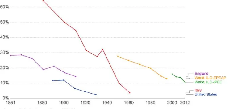
im-proved productivity and fostered economic development. The highly successful countries of

today increased their stock of human capital and infrastructure in the early stages of industrial

development, which increased household income and decreased the ratio of child labor (see

Figure 1). A lag delayed some countries from developing and setting up manufacturing, but

the fruits of prosperity were gradually realized (see Figure2). The countries with a significant

lag in prosperity are still suffering economically, and many children are involved in economic

activities (see Figure 3)1_{. Why has industrialization failed to make all countries rich, and}

why do large parts of the world still suffer from poverty? Because an increasing presence

of emerging country is expected to be a driving force in the global economy, identifying the

cause of stagnation and resolving it in less-developed countries has gained much attention.

Many studies have addressed the importance of infrastructure such as roads, bridges, public

transportation, and energy facilities on economic development (see for example, Calderon and

Chong (2004), Easterly and Rebelo (1993),Gramlich (1994), and Garcia-Mila, McGuire, and

Porter (1996) ) and show the positive correlation between the stock of infrastructure and

development (The World Bank (1994)). These types of infrastructure are known as

phys-ical infrastructure or public capital, and they improve the efficiency of economic activities.

Because economic growth can also shape the demand and supply of physical infrastructure

ser-vices, the underdevelopment of infrastructure is considered the cause of a lag in development

1_{The proportion of children aged between five and 17 years who work amounts to 19.6 % in Africa, 7.4}

(Esfahani and Ramirez-Giraldo (2003)). There is no doubt that the development of physical

infrastructure is central to economic development; however, other aspects of infrastructure,

such as the level of health care, education, and nutrition, also contribute to economic

devel-opment. For example, better public health improves the overall well-being of society because

healthier individuals are less myopic and tend to place greater value in the future2_{; healthy}

individuals prefer to acquire human capital (Jimenez (1995) and Bedi and Edwards (2002)).

This type of infrastructure classified apart from physical infrastructure and known as human

infrastructure (Jimenez (1995)). Human infrastructure increases the level of human capital

and productivity, which leads to higher wages, reduced child labor, and enhances investment

in human capital. The mechanism is expected to create a virtuous cycle endogenously, but

the analysis of the effect of human infrastructure on economic development has not received

much attention in existing literature. The analytical research on how the accumulation of

hu-man infrastructure affects economic development is extremely important to clarify the cause

of poverty and to find its solution. For this purpose, we set up a simple theoretical model

incorporating child labor and human infrastructure and investigate the causes of bifurcation

from an identical initial condition. By assuming that an increase in human infrastructure

im-proves the marginal productivity of labor, the first part of this paper analyzes the transition

dynamics to determine the reason why one economy can develop and another cannot despite

having the same initial condition. The second part of this paper investigates the possibility

of sustainable growth in developing countries. Because development aid is the main source

of support for less developed countries, and the amount of net official development assistance

is increasing year by year3_{, we examine the effect of development aid on poverty-stricken}

countries.

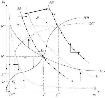
The remainder of this paper is organized as follows. Section 2 sets up the model. Section

3 characterizes the dynamic equilibrium path and analyzes the condition of divergence and

poverty. Section 4 analyzes the effect of development aid, and Section 5 concludes the paper.

2_{Agenor (2010).}

3_{US$6.817 billion (1970), US$34.475 (1980), US$58.242 (1990), US$49.804 (2000), US$130.685 (2010), and}

2

The Model

Consider an infinite-horizon economy composed of households, perfectly competitive firms,

and a government. A new generation of a unit mass, referred to as generation t, is born in

period t−1. Time is indexed by t= 1,2,· · ·. Generation t≥1 is composed of a continuum

of Nt units who live for three periods: childhood, adulthood, and oldhood.

Human Infrastructure

As noted by Jimenez (1995), human infrastructure can be classified separately from physical

infrastructure (transport, energy, water). It is defined as public capital that improves societal

levels of health status, education, nutrition, and labor productivity. Human infrastructure

also includes sanitation, environment, and legal and political institutional systems. When the

level of human infrastructure is considered as an indexgt, the level of human infrastructure in

period t+ 1gt+1 accumulates through investment in human infrastructure, iGt , and the level

of human infrastructure in the preceding period t gt:

gt+1 =iGt + (1−δ)gt, (1)

where δ∈(0,1) is the depreciation rate of human infrastructure.

Firms

In each period, there exists two potential sectors that are employed by Hazan and Berdugo

(2002). Production will take place in either one of them or in both. The existence of one sector

is independent of the existence of the other, and the existence of each sector is determined

by the optimal choices of individuals. Each sector produces consumption goods but employs

different factors: one sector employs only raw labor while the other employs efficiency units

of labor. We refer to the former as the “traditional sector” and to the later as the “modern

sector.” The production function of the traditional sector is ytra

t = ¯ylt, where ytra, ¯y, and

lt represent per capita output in the traditional sector, the productivity in the traditional

sector, and the quantities of raw labor, respectively. The wage rate in the traditional sector is

wtra _{= ¯y. The modern production function is given by y}mo

t =y(gt, ht) =ηφ(gt)ht, whereytmo,

η > 0, and ht, show per capita output in the modern sector, the level of technology, and the

augmented by the level of per capita human infrastructure where φ′

(gt)>0,φ

′′

(gt)<0, and

φ(0) = 0. The wage rate in the modern sector is set as wmo

t =ηφ(gt).

Government

We assume that government monitors child labor and human infrastructure investment. The

government levies income tax on adult agents4 _{and allocates it between two policy programs:}

child labor inspection and investment in human infrastructure. By assuming that whether a

firm employs children is private information, the government must inspect each firm to reveal

the extent of child labor by investing the costγ5. Inspection is not always successful, and the revealed child labor probability depends on the inspection cost π(γ) (0≤π(γ)<1) and also

has the properties: π′

(γ)>0, π′′

(γ)<0, π(0) = 0,limγ→∞π ′

(γ) = 0, and limγ→₀π ′

(γ) = ∞.

If the government can expose child labor, the company must pay a fine depending on the

amount that its child workers produce. Noting that the detection probability is π(γ), the

income from child labor iswc _{= (1−π(γ))¯y, and aggregate fines areπ(γ)¯yl}c

t wherelct shows the

amount of child labor. The fines are redistributed to non-returnable government investments

such as self-defense.6 _{The residual amount of tax income is allocated to human infrastructure}

investment: iG

t =Tt−γ7 whereTt shows aggregate tax revenue.

Individuals

The individuals of generation t are identical in their preferences. They live for three periods:

child, adult, and old period, with an endowed one unit of time in each period. The adult

agent (generation t) has a child and allocates their child (generation t−1) to either work lc t

or school et in period t. When parents send their children to work, children can earn wage

income wc

t. The sum of the time spent by children at work or in school must be unity, and

each value for time spent must lie between zero and unity in each period:

lc

t +et = 1, 0≤ltc ≤1, 0≤et ≤1. (2)

4_{Because child labor is a hidden action, the government cannot levy tax on child labor.}

5_{For example, the Ministry of Labor and Social Security in the Republic of Turkey introduced a program}

enforcing the supervision of child labor from 1994. As a result, the number of working children who were 15 years old or less decreased between 1997 and 1999 in Turkey (OECD (2003)) .

6_{When the fines are redistributed to investment in human infrastructure, we obtain the same results.} 7_{If we setγ=µT}

As in Galor and Weil (1996, 2000), and Holtz-Eakin, Lovely, and Tosun (2004), we assume

that the level of human capital is an increasing function of the time devoted to schooling et.

Additionally, the level of human capital is also an increasing and strictly concave function

of human infrastructure gt. For analytical tractability, we assume that individuals born in

period t obtain their human capital as follows:

ht+1 =h(et, ht)≡θetgσt, θ >0, 0< σ <1, (3)

where θ and σ express the parameters of education efficiency and the adjusted elasticity of

human capital with respect to educational level, respectively.

When an individual becomes an adult, that individual has children and decides whether

to donate all of their time to the traditional or modern sector. The decision is made according

to aggregate income: (1−τ)wtra_l

t and (1−τ)wtmohtlt. Noting that lt = 1, potential income

Yt is decided as follows,

Yt = max{(1−τ)wtra, (1−τ)wtmo}. (4)

When parents consume all of their family income; that is, their own income and that of

their children, we have a budget constraint for that adult as follows:

ct=Yt+ (1−π(γ))wtcl c

t. (5)

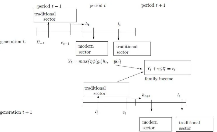
Figure 4 shows a sketch of the relationship between each generation.

An individual from generation t has preference over their consumption ct and the level of

human capital of their children ht+1. We assume the following utility function:

Ut= logct+βloght+1, (6)

where β ∈(0,1) indicates the degree of altruism by parents toward their children.

At each time point, adult individuals first decide their occupation by comparing the income

of both sectors and then allocating their children’s time by maximizing (6) subjects from (4) to

(5). Hence, for given levels of wtra_,wmo

t , andwc, the optimization problem of each individual

of generation t can be expressed as follows:

max

lt

Ut = log{Yt+ (1−π(γ))wcltc}+βlog{θ(1−lt)gtσ},

The first-order condition with respect to lt is given by

∂Ut

∂lc t

= (1−π(γ))w

c t

Yt+ (1−π(γ))wctlct

− β 1−lc

t

S0, (with equality if 0< ltc <1). (7)

The first and second terms on the right-hand side of (7) represent the marginal benefit and

the marginal cost of child labor.

3

Equilibrium

In this section, we examine the equilibrium and dynamic system of the economy.

3.1

Equilibrium

At first, the adult individual makes the occupational choice by comparing an expected income.

Substituting the wage rate into (4), the individual who satisfies ht≤y/ηφ(g¯ t)≡hchooses an

occupation in the traditional sector and ¯h≤ht chooses an occupation in the modern sector.

Next, the individual maximizes their utility by choosing the working time of their children.

Noting the individual who has h ≤ ht work in the modern sector, we obtain the following

equilibrium relationship between child labor and human capital:

lct(ht, gt)≡lct =

          

1−π(γ)−β(1−τ)

(1 +β)(1−π(γ)) if ht ≤h, (1−π(γ))¯y−β(1−τ)ηφ(gt)ht

(1 +β)(1−π(γ))¯y , if h≤ht ≤¯h,

0, if ¯h≤ht,

(8)

where h ≡ _ηφy₍¯_gt) and ¯h ≡ (1−π(γ))¯y

β(1−τ)ηφ(gt). (8) show that the time spent working by children

depends on the level of human capital of the child’s parents. When the level of human capital

is sufficiently low, parents cannot earn sufficient income to survive and have to rely on their

children for income.

3.2

The Dynamic Equilibrium Path

From (2), (3), and (8), we obtain the dynamics of human capital as follows:

ht+1 =

          

θβ(2−τ −π(γ)) (1 +β)(1−π(γ))g

σ

t, if ht≤h,

θβ((1−π(γ))¯y+ (1−τ)ηφ(gt)ht)

(1 +β)(1−π(γ))¯y g

σ

t, if h≤ht≤¯h,

θgσ

t, if ¯h≤ht.

Accordingly, investment in human infrastructure is decided as

iG t =

(

τy¯−γ, if ht≤h,

τ ηφ(gt)ht−γ, if h≤ht,

(10)

where γ is the inspection cost of child labor. By using (1), (8), and (10), we obtain the

following:

gt+1 =

(

(1−δ)gt+τy¯−γ, if ht≤h,

(1−δ)gt+τ ηφ(gt)ht−γ, if h≤ht.

(11)

(9) and (11) show the system of this economy and indicate that the dynamics systems of the

economy are completely described by these difference equations inhtandgt. Before analyzing

the equilibrium, we consider the borderline between the regimes. For analytical tractability,

we impose8

φ(gt) = gt. (12)

This leads to the borderline relations: h and ¯h are as follows:

h ≡ ht=

¯ y ηgt

, (13)

¯

h ≡ ht=

(1−π(γ))¯y β(1−τ)ηgt

. (14)

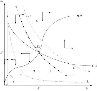
By using (9), (11), (13), and (14), we can draw the phase diagram on the (ht, gt) plane.

We refer to the locus on the (ht, gt) plane, representing ht+1 = ht as HH locus and that

representing gt+1 = gt as GG locus. The HH and GG loci represent equal parts of (9) and

(11), respectively. By applying (12), we have a complete dynamic systems as follows:

ht+1 ≥ht⇔

ht≤

          

θβ(2−τ−π(γ)) (1 +β)(1−π(γ))g

σ

t ≡H0(gt), if ht ≤h,

θβ(1−π(γ))¯ygσ t

(1 +β)(1−π(γ))¯y−θβ(1−τ)ηg1+σ t

≡H1(gt), if h≤ht ≤¯h,

θgσ

t ≡H2(gt) if ht ≥¯h,

(15)

gt+1 ≥gt⇔ gt≤

τy¯−γ

δ ≡G0, if ht≤h ht ≥

δgt+γ

τ ηgt

≡G1(gt), if h≤ht, (16)

8_{If we imposeφ(g}

H1(gt) and H2(gt) in (15) satisfies dH1/dgt >0, limg→g∂H1/∂gt = 0, limgt→g¯∂H1/∂gt= ∞9

and ∂H2/∂gt>0, ∂2H2/∂gt2 <0. Additionally, G1(gt) in (16) also satisfies∂G1/∂gt<0 and

∂2_G

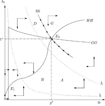
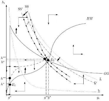
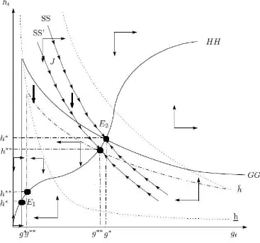
1/∂gt2 >0. The phase diagrams in the economy are shown in Figure 5 and Figure 6. For

simplicity, we denote the saddle path described in Figure 5 and 6 as the SS curve. Because

ht and gt are state variables, their initial values h0 and g0 are historically given, and the

economies that are initially on the SS curve converge to the steady-state equilibrium. The

steady-state equilibrium (h∗

, g∗

) is at the intersection of the HH and GG locus. There exist

two possible equilibria, and the next lemma summarizes the differences of these equilibria.

Lemma 1 Suppose thatη >(<)¯η, the high steady-state equilibrium is in the regime without

(with) child labor; that is, ¯h≤ht(h≤ht≤¯h). where η¯= (1

−π(γ))¯y θβ(1−τ)η(

τ(1−π(γ))¯y−γβ(1−τ) δβ(1−τ) )

−_(1+σ)

.

Proof. When the equilibrium is in the regime ¯h < ht, the intersect point ofH1(gt) (equation

(15) and ¯h is larger than the intersect point G1(gt) (equation (16)) and ¯h. Now, we define

the previous intersect point as gh _{and the latter asg}g_{. Thus, we have}

gh _≡(1−π(γ))¯y

θβ(1−τ)η

₁₊1σ

> τ(1−π(γ))¯y−γβ(1−τ) δβ(1−τ) ≡g

g_.

By arranging the equation, it becomes η > η¯ ≡ (1−_π(γ)¯y

θ(1−τ)

τ(1−_π(γ)¯y−_γβ(1−_τ)

δβ(1−τ)

−_(1+σ)

. When

productivity is high, the economy has low steady-state equilibrium and vice versa.

High productivity decreases the marginal benefit from child labor and decreases child labor in

the long run. As a result, the economy with higher productivity experiences the steady-state

equilibrium without child labor. The next proposition shows the stability of the equilibrium.

Proposition 1 There exists multiple equilibrium (E1 and E2). The higher equilibrium E2 is

a saddle point stability and satisfies the following:

η <η¯ : (g∗

)1+στ ηθβ(1−π(γ))¯y= (δg∗

+γ)((1 +β)(1−π(γ)¯y)−θβη(1−τ)(g∗

)1+σ),

η >η¯ : τ ηθ(g∗

)1+σ =δg∗

+γ.

Proof. See Appendix.

A case where the economies are initially on the SS curve is rare. In general, an economy

9_{g→g¯≡(1 +β)(1−π(γ))¯y/γβη(2−τ−π(γ)))}1/(1+σ) _{shows the level ofg that satisfiesH}

1(gt) =h, and

¯

g≡(γβ(2−τ−π(γ))/(1 +β)(1−π(γ)))σ _{shows the level ofgthat satisfies H}

is endowed with (h0, g0) above or below the SS curve. If (h0, g0) is at the point below the

SS curve, such as the point B (low level of human capital and human infrastructure) in

Figure 5 and Figure 6, the output is too low for workers to earn sufficient wages and to

invest in human infrastructure. Because wage incomes are low, parents must rely on their

children to supplement family income, which results in diminished accumulation of human

capital. Lower human capital prevents workers from entering the modern sector and results

in fewer resources invested in human infrastructure and lower productivity levels and wage

rates. These mechanisms create a vicious cycle, and the economy finally converges to the

poverty trap equilibrium. On the other hand, if (h0, g0) is at a point above the SS curve,

such as point G (a high level of human capital and human infrastructure) in Figure 5 and

Figure 6, output and human capital are sufficient for workers to earn sufficient wages. A

high wage released children from the need to work and enhances the government’s ability to

invest in human infrastructure. A high wage also improves the productivity of human capital

and wage rates. These mechanisms create a virtuous cycle, and the economy can perform

sustainable development.

Next, we examine the case where initial endowments isD in Figure 5 and Figure 6. Note

that the economy that has the same initial endowments has completely different dynamics.

One economy in Figure 6 experiences sustainable growth, the other economy in Figure 5 falls

into the poverty trap. The next proposition summarizes the results.

Proposition 2 Even if initial conditions are the same, whether the economy continues to

achieve economic growth depends on productivity. When productivity is high enough, the

economy can sustain long-run growth.

As noted, when productivity is high, individuals receive higher wages, and they do not rely

on their children for family income. Additionally, higher wages increase the tax income of

government and results in greater investment in human infrastructure. This creates a virtuous

cycle, and the economy experiences sustainable growth.

3.3

Numerical Simulation

The purpose of the paper is to construct a theoretical model that explains the historically

of these dynamic equilibrium paths, we used numerical calibrated version simulations of the

model. For illustrative purpose, we parameterized the function π(γ) as π(γ) =αγ/(1 +αγ)

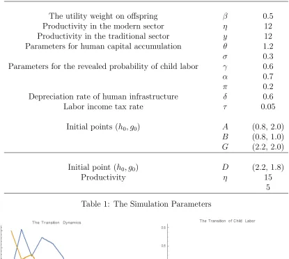
where α ∈ (0,1). The parameters used in the baseline simulation are given in Table 1.

Treating each period as 25 years, we calculated the equilibrium values for the 10 periods from

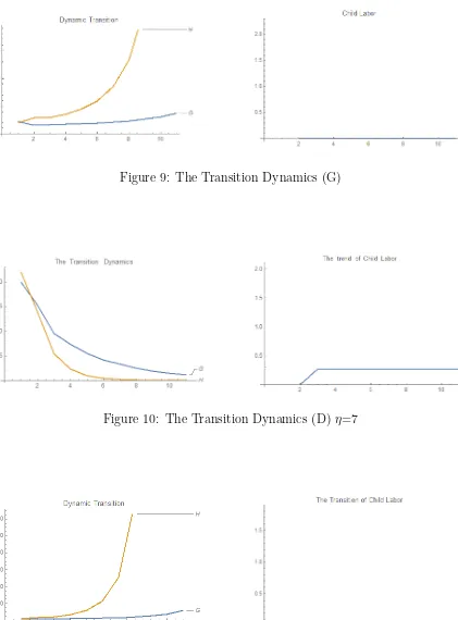
1750 to 2000. Figure 7 to Figure 11 show the numerically analyzed transition paths of human

capital h, human infrastructure g, and child labor lc_{, respectively, where the initial level of}

stocks are the points A, B, G, and D in Figure 5 and 6. These paths show that when the

initial point starts below (above) the SS curve, the transition dynamics of g and h fall into

the vicious cycle (diverge). Figure 7 shows the transition of the vicious cycle. In the economy,

low accumulation of human capital and social infrastructure increases the level of child labor.

These trends indicate the economy cited in Figure 3. Moreover, the economy in Figure 1 and

2 can be adapted in the economy of Figure 9 and Figure 8, respectively. For these paths,

the accumulation of human infrastructure creates a vicious cycle and increases the level of

child labor. Figure 10 and 11 show the transition path with the same initial condition. As

proposition 2 showed when productivity is low, the economy converges to a lower level of the

steady-state equilibrium.

4

The Effect of Foreign Development Assistance

This section investigates the effect of development assistance on recipient countries. Currently,

aid is the main source of support to less-developed countries, and international organizations

such as the United Nations and The World Bank support these countries through multiple

schemes (The World Bank (2009))10_{. One of the main schemes is a child protection program.}

Because child labor prevents children from obtaining an education and hinders their physical

and mental development, the eradication of child labor is one of the goals of child

protec-tion. The other scheme is development aid whereby rich countries support poor countries by

investing in infrastructure.

We examine how these tied aids influence individual decision making and steady-state

equilibrium in recipient countries. First, we examine the effect of the child protection program.

To eradicate child labor, this aid strengthens the inspection of child labor by increasing the

10_{Particularly, the International Labor Organization and The World Bank jointly provide poverty}

inspection cost from γ to γ′

= γ +a where a shows the total amount of aid distributed to

each developing country. Because the program decreases the marginal utility of child labor,

it decreases the incidence of child labor and contributes to increased human capital. The aid

also shifts HH loci upwards as follows:

ht+1 ≥ht⇔

ht ≤

          

θβ(2−τ −π(γ′

)) (1 +β)(1−π(γ′

))g

σ t ≡H

′

0(gt), if ht ≤h,

θβ(1−π(γ′

))¯ygσ t

(1 +β)(1−π(γ′_{))¯y−θβ(1−τ)ηg}1+σ

t

≡H′

1(gt), if h≤ht ≤¯h,

θgσ t ≡H

′

2(gt) if ht ≥¯h,

Aid from the child protection program also shifts the ¯hline (equation (14)) downwards. Figure

12 shows the effect of aid on the dynamics, and the dotted line shows the dynamics with aid.

The aid increases (decreases) the steady-state level of human capital of E1(E2), decreases

the level of human infrastructure of E2, and shifts the SS line downwards. Therefore, the

economy that initially occurs on the regime betweenSS and SS′

curve (see pointJ in Figure

12) has the potential for long-run growth. The child protection program has two effects on

the steady-state welfare level. One is an income effect because the child protection program

decreases the child labor in terms of time. However, this leads to lower levels of family

income and consumption. Thus, the income effect has a negative effect on the steady-state

welfare level. The other effect is an education effect, the child protection program encourages

education and increases the stock of human capital. Thus, the education effect has a positive

effect on the steady-state welfare level. The overall effect on welfare depends on the level

of human infrastructure. When the level of human infrastructure is high, the positive effect

dominates the negative effect and vice versa.

Next, we examine the effect of development aid. Development aid supports the

accumu-lation of human infrastructure and changes investment as iG

t = Tt−γ to iG ′

t = Tt−γ+a.

The GG loci will be amended as follows:

gt+1≥gt⇔ gt ≤

τy¯−γ+a δ ≡G

′

0, if ht≤h

ht≥

δgt+γ−a

τ ηgt

≡G′

1(gt), if ¯h≤ht,

The aid does not have a direct effect on the accumulation of human capital, but it indirectly

increases human capital. With the new dynamics, the G′

steady-state level of human capital and human infrastructure increase. The shift in line G′

1

depends on the level of aida. Whenγ > a,G′

1 shifts downwards (see Figure 13), this results in

a low steady-state equilibrium for human capital and human infrastructure. The SS line also

shifts downwards; however, the economy that initially occurs on the regime between SS and

SS′

curve (see point J in Figure 13) also has the potential for long-run growth. On the other

hand, when γ < a, G′

1 shifts upwards (see Figure 14), this results in a higher steady-state

equilibrium for human capital and human infrastructure. The SS line also shifts upwards,

and the economy that initially occurs on the regime between theSS andSS′

curve (see point

J in Figure 14) misses the potential for development. Development aid also has two effects;

consumption effect and education effect. For the lower steady-state equilibrium (E1) where

parents work in the traditional sector, the aid does not have a direct effect on family income.

The aid indirectly increases the level of human capital, which positively affects the

steady-state welfare level. For the higher steady-steady-state equilibrium (E2) where the parents work in

the modern sector and employ child labor, the effect of aid on welfare depends on the level

of aid. When the level of aid is sufficiently large, a decrease in the marginal utility of child

labor reduces the level of child labor. However, the increased stock of human infrastructure

enhances the adult income and results in a positive income effect on the steady-state welfare

level. The more the level of human infrastructure enhances the stock of human capital, the

more positive the effect of human capital on the steady-state welfare level. When the level

of aid is sufficiently low, a decrease in the marginal utility from child labor reduces the level

of child labor. Because the aid increases the level of human infrastructure and the income

of parents, the aggregate income effect on the steady-state welfare level is ambiguous. The

aid also has a negative human capital effect on the steady-state welfare level. Therefore,

the overall effect on welfare is ambiguous. The sufficiently large level of aid is generous for

development aid. However, as we noted before, the economy that initially occurs on the SS

line is rare. The majority of economy are initially endowed with (h0, g0) above or below the

SS curve. Particularly for economies initially endowed between the SS and SS′

line, aid

is detrimental to the economy. Therefore, when the income of the recipient country is not

extremely low but there is child labor, the aid to prevent child labor is more effective than

When child labor is conspicuous, the aid that reduces child labor is considered more

effective than aid to enhance infrastructure. Because the direct reason for child labor is

poverty, and families rely on their children for income, aid designed to prevent child labor

is detrimental to welfare. Although development aid may not seem directly related to the

eradication of child labor, it has the effect of enhancing adult income and results in low levels

of child labor.

5

Conclusion

The average person in year 1800 was no better off than the average person in 100,000 BC.

However, the Industrial Revolution that occurred two hundred years ago irrevocably changed

the possibilities for material consumption. Incomes per person reached a phase of sustained

growth in a favored group of countries. The richest modern economies are now 10 to 20

times wealthier than the average economy in the year 1800. Prosperity, however, is not

enjoyed by all societies. Material consumption in some countries, mainly in sub-Saharan

Africa, is now well below pre-industrial levels. Why did industrialization fail to benefit the

whole world? Why did it make substantial areas of the world even poorer? To address

these questions, this paper constructs a simple theoretical model, which incorporates human

infrastructure and child labor. In the first part of the paper, we show that when the economy

has the same initial condition, the economy with a high level of technology exhibits sustainable

growth. However, the economy with a low level of technology falls into the poverty trap. In

addition, we show the historically observed trends in child labor and development. The second

part of the paper examines the effect of development assistance in recipient countries. By

comparing development assistance programs that call for the elimination of child labor and

the strengthening of human infrastructure, we find that aid for the elimination of child labor is

effective for middle-income countries, and aid to strengthen human infrastructure is effective

Appendix

Appendix A

We examine the stability of the equilibriums E1 and E2. To examine the local dynamics

of equilibrium E1 (or E2), we take a first-order Taylor expansion of the system around the

E1 = (h∗, g∗). Noting that ˇht≡ht−h∗ and ˇgt ≡gt−g∗, the linearizing of equations (9) and

(11) in the equilibrium E1 is expressed as:

_ˇ

ht+1

ˇ gt+1

=

Ω(g∗

)1+σ Ω(X(g∗

)σ−₁

+ (1 +σ)ηh∗

(g∗

)σ) τ ηg∗

1−δ+τ ηh∗

ˇ ht

ˇ gt,

where g∗

and h∗

are shown in proposition 1; and Ω ≡ θβ(1−τ)η

(1+β)(1−π(γ))¯y and X ≡

σ(1−π(γ)¯y (1−τ)η . The

characteristic polynomial becomes:

P(κ) =κ2−T κ+D,

T = Ω(g∗

)1+σ + 1−δ+τ ηh∗

>0,

D = Ω(g∗

)1+σ(1−δ+τ ηh∗

)−Ωτ ηg∗

(X(g∗

)σ−₁

+ (1 +σ)h∗

(g∗

)σ).

Azariadis (1993) checks that the steady state is a saddle point, whenP(1)<0 andP(−1)>0

hold simultaneously.

P(1) = 1−Ω(g∗

)1+σ _{−(1−δ+τ ηh}∗

) + Ω(g∗

)1+σ_{(1−δ+τ ηh}∗

)−τ ηΩ(g∗

)(X(g∗

)σ−₁

+ (1 +σ)h∗

(g∗

)σ₎

= (1−Ω(g∗

)1+σ_{)(δ−τ ηh}∗

)−τ ηΩ(g∗

)(X(g∗

)σ−₁

+ (1 +σ)h∗

(g∗

)σ_).

Now, we suppose that 1 −Ω(g∗

)1+σ _{= 1−} θβ(1−τ) (1+β)(1−_π(γ))¯y(g

∗

)1+σ _{< 0. To hold this}

assump-tion, (g∗

)1+σ _{should be larger than} (1+β)(1−π(γ))¯y

θβη(1−τ) . Although Lemma 1 shows the steady-state

equilibrium is in the regime (g∗

)1+σ _< (1−π(γ))¯y θβη(1−_τ) ≡ g

h_{, because} (1−π(γ))¯y θβη(1−_τ) <

(1+β)(1−π(γ))¯y θβη(1−_τ) , the

assumption is contradicted.

Next, we examine the sign of δ −τ ηh∗

. Substituting the equilibrium value h∗

= (δg∗

+

γ)/τ ηg∗

(see equation (16) in the previous equation,δ−τ ηh∗

=−τ ηγ <0, we haveP(1)<0.

p(−1) = 1 + Ω(g∗

)1+σ _{+ 1−δ+τ ηh}∗

+ Ω(g∗

)1+σ_{(1−δ+τ ηh}∗

)−τ ηΩX((g∗

)σ_{−(1 +σ)τ ηΩh}∗

(g∗

)1+σ_),

= 1 + Ω(g∗

)1+σ _{+ 1−δ+ Ω(g}∗

)1+σ_{(1−δ) +τ ηh}∗

−τ ηΩX((g∗

)σ_{−στ ηΩh}∗

(g∗

Substituting the equilibrium value of h∗

(see 15), we have

τ ηh∗

−τ ηΩX((g∗

)σ −στ ηΩh∗

(g∗

)1+σ)

= τ ηθβ(g

∗

)σ

(1 +β)(1−π(γ)¯y−θβ(1−τ)η(g∗

)1+σ(1−σ)(1−π(γ)¯y(1 +β) 2 _>0.

Therefore, we have P(1)<0 and P(−1)<0.

Next, we examine the local dynamics of equilibriumE2 = (h∗, g∗). Using the same

proce-dure, the linearization of equations (9) and (11) in the equilibrium E2 is expressed as:

ˇ

ht+1

ˇ gt+1

=

0 σθ(g∗

)σ−₁

τ ηg∗

1−δ+τ ηh∗

ˇ ht ˇ gt .

T = 1−δ+τ ηh∗

>0, D=σθ(g∗

)σ−₁

τ ηg∗

>0.

Since P(−1) = 1 +T +D > 0 and P(1) = δ−τ ηh∗

−σθτ η(g∗

)σ_{. Because δ −τ ηh}a_{st =}

−gamma/g∗

<0,P(1) <0. Therefore, E2 is a saddle stable equilibrium.

References

Agenor, P.-R. (2010): “A theory of infrastructure-led development,” Journal of Economic Dynamics and Control, 34(5), 932–950.

Azariadis, C. (1993): Intertemporal Macroeconomics. Basil Blackwell, Oxford.

Bedi, A., and J. Edwards (2002): “The impact of school quality on earnings and educa-tional returns–evidence from a low-income country,” Journal of Development Economics, 68(1), 157–185.

Calderon, C., and A. Chong (2004): “Volume and Quality of Infrastructure and the Distribution of Income: An Empirical Investigation,”Review of Income and Wealth, 50(1), 87–106.

Clark, G. (2008): A Farewell to Alms: A Brief Economic History of the World. Princeton Press.

Easterly, W., and S. Rebelo(1993): “Fiscal policy and economic growth: An empirical investigation,”Journal of Monetary Economics, 32(3), 417–458.

Esfahani, H., and M. Ramirez-Giraldo (2003): “Institutions, infrastructure, and eco-nomic growth,”Journal of Development Economics, 70(2), 443–477.

Galor, O., and D. N. Weil (1996): “The Gender Gap, Fertility, and Growth,” American Economic Review, 86(3), 374–87.

Garcia-Mila, T., T. J. McGuire, and R. Porter (1996): “The Effect of Public Cap-ital in State-Level Production Functions Reconsidered,” The Review of Economics and Statistics, 78(1), 177–80.

Gramlich, E. M. (1994): “Infrastructure Investment: A Review Essay,” Journal of Eco-nomic Literature, 32(3), 1176–96.

Hazan, M., and B. Berdugo (2002): “Child Labour, Fertility, and Economic Growth,”

Economic Journal, 112(482), 810–828.

Holtz-Eakin, D., M. E. Lovely, and M. S. Tosun(2004): “Generational conflict, fiscal policy, and economic growth,” Journal of Macroeconomics, 26(1), 1–23.

ILO (2017): Global estimate of child labour: Results and trends, 2012-2016. International Labour Organization.

Jimenez, E. (1995): Human and physical infrastructure: Public investment and pricing policies in developing countries, vol. 3 ofHandbook of Development Economics. Elsevier.

OECD (2003): Combating Child Labour: A Review of Policies. Organization for Economic Co-operation and Development.

Ortiz-Ospina, E., and M. Roser (2018): “Child Labor,”OurWorldInData.org, Available from https://ourworldindata.org/child-labor.

The World Bank (1994): World Develop;ment Report 1994: Infrastructure for Develop-ment. Oxford University Press.

(2009): Country Assistence Strategies: Retrospective and Future Directions. Opera-tions Policy and Country Services, World Bank.

Figure 1: Child Labor Trends in Developed Countries

Figure 3: Child Labor Trends in less-developed Countries

Description Parameter Value

The utility weight on offspring β 0.5 Productivity in the modern sector η 12 Productivity in the traditional sector y 12 Parameters for human capital accumulation θ 1.2

σ 0.3

Parameters for the revealed probability of child labor γ 0.6

α 0.7

π 0.2

Depreciation rate of human infrastructure δ 0.6 Labor income tax rate τ 0.05

Initial points (h0, g0) A (0.8, 2.0)

B (0.8, 1.0) G (2.2, 2.0)

Initial point (h0, g0) D (2.2, 1.8)

Productivity η 15

5

Table 1: The Simulation Parameters

Figure 7: The Transition Dynamics (A)

Figure 9: The Transition Dynamics (G)

Figure 10: The Transition Dynamics (D) η=7