Munich Personal RePEc Archive
Income inequality, consumption, credit
and credit risk in a data-driven
agent-based model
Papadopoulos, Georgios
Analysis and Research Centre, Bank of Slovenia
30 October 2018
Online at
https://mpra.ub.uni-muenchen.de/89764/
Income inequality, consumption, credit and credit
risk in a data-driven agent-based model
Georgios Papadopoulos
∗Analysis and Research Centre, Bank of Slovenia, Ljubljana,
Slovenia
[email protected]
Abstract
The issue of income inequality occupies a prominent position in the research agenda of academic and policy circles alike, especially after the crisis of 2008, due to its potential causal link with the development of credit bubbles and therefore the emergence of financial crises. This pa-per examines the long-run effect of income inequality on consumption, consumer credit and non-performing loans through the means of a data-driven agent-based model. The data-data-driven nature of the model enhances its ability to match historical series and thus makes it suitable for policy simulations tailored for specific economies. The analysis indicates that higher income inequality has a detrimental impact on consumption and is associated with lower volumes of consumer credit. However, the ratio of non-performing loans as a share of total loans seems to be independent of income inequality.
JEL classification: C63; D31; E21; E27
Keywords: Income inequality; Consumption; Consumer credit;
Non-performing loans; Agent-based model
∗The idea for this project was conceived while the author was attending Santa Fe Institute’s
1
Introduction
The central theme of this paper is the effect of inequality in the distribution of income on aggregate macroeconomic and financial variables. At its core is
essentially a thought experiment attempting to answer the question: How would
the initial level of income inequality affect aggregate consumption, consumer credit and non-performing loans of an economic system which would otherwise follow a specific historical scenario?
The issue of inequality and the effects of its various manifestations -such as income, wealth or consumption- on both developing and developed countries has
attracted the attention of academia and policy makers alike1, especially after
the financial crisis of 2008, with several studies documenting significant increases in the skewness and kurtosis of income and wealth distributions over the past three decades (e.g. Piketty and Saez (2003, 2006), Atkinson and Morelli (2011)). However, this topic might not have risen to such prominent position within the economics profession if it weren’t for the potential causal links between rising inequality and financial crises.
The rationale behind this cause and effect relationship begins with house-holds with insufficient financial resources resorting to borrowing in order to maintain their living standards. In turn, the excess leverage creates unsustain-able credit growth which subsequently ends with a credit bubble bust. One of the consequences of the latter is the amplification of pre-existing inequalities thus resulting in a positive feedback loop between inequality and crises. For a review of the recent literature on the complex interconnections between inequal-ity, leverage and crises the reader is referred to the excellent work of Bazillier and H´ericourt (2017) and references therein.
Interestingly, empirical literature on the first, fundamental element of the hypothesized underlying mechanism linking higher inequality with increased volumes of credit is not conclusive. Results range from suggesting a positive (Christen and Morgan, 2005; Perugini et al., 2015), negative (Coibion et al., 2014) or even non-significant (Bordo and Meissner, 2012) relationship. On the contrary, theoretical works display a higher consensus regarding the sign and the direction of the aforementioned relationship. Contributions from the DSGE literature (Iacoviello, 2008; Kumhof et al., 2015) show how increased inequality can create highly indebted, low-income households which eventually results in a fragile economy, prone to financial and real crises.
Another strand of literature employs agent-based models (ABM)2to explore
the economic effects of various inequality forms such as income (Cardaci and Saraceno, 2015; Dosi et al., 2013, 2015, 2016; Palagi et al., 2017), wealth (Russo et al., 2016) or both (Caiani et al., 2017) and indeed finds that higher inequality has detrimental macroeconomic effects, impeding growth and increasing the
1
For the latter see Amaral (2017), Colciago et al. (2018) or Ampudia et al. (2018) and references therein for studies on the relationship between central bank policies and inequality.
2
probability of a crisis occurring.
The bottom-up nature of ABM makes this approach flexible and appropriate to examine distributional questions, hence it will be followed in this study. However, contrary to the aforementioned works where fully-fledged models are developed with all interactions among agents being endogenously determined, in this paper certain agents are not explicitly modelled. Instead, for simplicity, their interactions with the other agents enter the model exogenously, as input
from historical data3 (Hassan et al., 2010).
This modelling choice allows to simplify the interaction structure among agents to a large extent by forcing them to follow as closely as possible the actual evolution of several key variables. This specific approach has two benefits. Firstly, it enables the targeted examination of the effect of a single parameter, namely income inequality, on the variables under study. Secondly, it permits to bring the model closer to the data than the current standard in the ABM
literature in economics which is the replication of empirical regularities.4 By
doing so, the empirical validation of the model extends beyond matching stylized facts between simulated and actual data, to directly comparing the evolution of the historical with the artificially generated time series. This enables to use the model for policy simulations referring to specific economies, in addition to answering the core question on the impact of the initial level of income inequality on macro-financial variables.
The remainder of the paper is organized as follows. In section 2 the model’s structure is described in detail. Agents’ behavioural rules and interactions in the various markets are elaborated, including a crucial element which is their expectations formation mechanism. Section 3 initially describes the input data used and presents the outcome of model’s validation before proceeding with the presentation and discussion of the simulation results. Finally, section 4 concludes exploring potential uses and extensions of the model.
2
The model
This section provides a description of the modelling properties which charac-terise the agent-based, macroeconomic model under development. The most
elaborate agents of the economic system are households (h = 1,2, ..., H) and
banks, represented as an all-encompassing banking sector agent. For the re-maining agents such as firms, the central bank and the government historical data are used to determine the evolution of their interactions with the former
3
Thus, it is closely related to the ”history-friendly” approach to calibration identified by Fagiolo et al. (2007).
4
agents in the respective markets.
The economic system evolves overt= 1,2, ..., T time periods, withT being
determined by the time range of the historical data used. As follows from the focus of agents’ development, the most detailed market in which they interact is the credit market. All other markets are passive and their evolution is governed by that of the historical series.
Households are boundedly rational and simple heuristics control their be-haviour. If their financial position allows them, they consume a proportion of their expected income and past deposits in each period and save any remaining resources. Otherwise, in case they are in financial distress, they consume a min-imum amount or they ask for credit if their financial position is sound. A key role in credit demand is played by the households’ income expectations forma-tion mechanism. Based on the heuristics switching model (HSM) of Anufriev and Hommes (2012a,b), households follow simple linear, adaptive and trend ex-tracting rules to form their expectations. In addition, their chosen rule is not fixed but they update their selection from a small pool of expectation heuris-tics according to their past performance. As pointed out by De Grauwe and Macchiarelli (De Grauwe and Macchiarelli, 2015) it is indeed rational to utilize simple forecasting heuristics and monitor their performance given one’s limited cognitive capabilities.
On the supply-side of credit, the bank bases its decision to provide credit on its available deposits and a time-variant measure proxying its risk tolerance, namely the debt service to income ratio (DSTI).
Finally, the labour market is entirely data-driven. The monthly evolution of households’ income and their employment status enter the model as input from historical data. Households’ income, there being no explicitly modelled gov-ernment agent and thus no taxes, corresponds to their disposable income. For
brevity, in the remainder of the paperincome will be used to refer to disposable
income. Unemployed households receive an unemployment benefit from the gov-ernment which is assumed to coincide with the subsistence consumption level. It should be noted that the only interaction between the implicit government agent and households is through the unemployment benefit.
In the following subsections are described the initialization of the simulation, the timeline of events taking place at each period and subsequently the agents and their interactions in the respective markets.
2.1
Initialization
One of the prerequisites for a micro-founded ABM is that agents’ initial con-ditions should be initialized with actual data (Delli Gatti et al., 2011). At the
beginning of the simulation each household is endowed with a monthly income5
drawn from a gamma distribution, Γ(α,1/λ) withαandλthe shape and scale
5
parameters respectively.6 By adjusting the shape and scale one can specify the distribution so that it has the same average and minimum values as well as the same degree of inequality as the historical distribution. It should be noted that,
for a givenα, the smaller theλthe less skewed the distribution, i.e. the lower
the inequality.
The initialization of the unemployment rate is also based on its historical figures at the start of the simulation. According to these, a number of households is chosen randomly and their income is fixed at the level of the unemployment dole which permits them to maintain the minimum consumption level required to survive.
After the initialization of income and unemployment all growth rates are set
to zero and the simulation is executed for a burn-in period of N time steps,
after which the system is assumed to have reached its equilibrium. After that period the historical data enter into the model and its output is recorded.
2.2
Sequence of events
The sequence of events in every period of the simulation is the following:
1. Historical series for income and unemployment growth as well as loan and deposit interest rates are updated.
2. The bank sets its DSTI level.
3. Households collect the interest from any deposits they have placed at the bank.
4. Employed households receive their monthly income based on the afore-mentioned historical growth rates.
5. The historical evolution of unemployment determines households’ employ-ment status.
6. Households update their income expectations.
7. Households address their financial obligations and determine their desired consumption.
8. Households with insufficient own financial resources to meet their desired consumption ask for credit.
9. The bank calculates and offers the maximum amount of credit it can to a household given its DSTI and the income of the latter.
10. Households meet their desired consumption or a fraction of it in case they are financially constrained and deposit any remaining income.
6
2.3
Agent and market description
This subsection provides a detailed description of the agents, their behavioural rules and interactions in the various markets.
2.3.1 Households
Households’ consumption decisions crucially depend on their financial position and in particular their ability to consume the minimum amount which ensures their survival. This is summarized in the following rule:
Cd
h,t=
(
Cmin,t, Ih,t+Dh,t−1< LPh,t+Cmin,t
max{αy·Ih,t+1e +αw·Dh,t−1, Cmin,t}, Ih,t+Dh,t−1≥LPh,t+Cmin,t
(1)
with 0< αw< αy <1 the marginal propensities to consume out of wealth
and income respectively.
Those households whose sum of current income (Ih,t) and past deposits
(Dh,t−1) does not suffice for them to consume the minimum amount (Cmin,t)
and meet their monthly loan payment (LPh,t), set their desired consumption
(Cd
h,t) to that of the subsistence level. It follows that they don’t service any
loans they might have for as long as these conditions remain. On the contrary, households who can afford minimum consumption and service their loan they do so and set their desired consumption as the largest element between a percentage
of their expected income (Ih,t+1) and past deposits ande Cmin,t.
The specific Modigliani (Modigliani and Brumberg, 1954) consumption func-tion of the financially sound households in Equafunc-tion (1) is thoroughly discussed in Godley and Lavoie (2016) and is widely used by the respective ABM litera-ture (Delli Gatti and Desiderio, 2015; Gualdi et al., 2015; Ricetti et al., 2013; Riccetti et al., 2015; Assenza et al., 2015; Caiani et al., 2016; Russo et al.,
2016; Gurgone et al., 2018; Meijers et al., 2018, among others).7
Although such rule may seem overly simple, Allen and Carroll (2001) argue that linear, rule-of-thumb consumption functions can indeed provide a good approximation of consumption functions -such as the one from buffer stock theory- derived as solutions to utility maximization problems. One interesting implication of the linear consumption function of Equation (1) is that households have a target
wealth to income ratio of (1−αy)/αw. Therefore, in an attempt to reach it, they
save when their target level of wealth is higher than the realized one (Godley and Lavoie, 2016).
In case a household’s remaining income and deposits (i.e. after servicing its loan) is enough to meet its desired level of consumption, it uses its own financial resources (withdrawing from its deposits if need be) to satisfy it. Otherwise it asks for consumer credit from the bank. A household asking for credit is assumed to spend any amount granted along with all of its income plus deposits
7
to satisfy its desired consumption. Thus, it may consume less or more than desired depending on the supplied credit.
Finally, after consumption plans are executed, any income remaining is de-posited at the bank at the given overnight deposit interest rate.
2.3.2 Expectations formation
Due to the pivotal role expectations play in credit demand in the model, their formation mechanism merits an elaborate description.
Research on expectations formation has identified three key facts regarding individuals’ behaviour:
• Expectations are heterogeneous among individuals.
• Individuals use simple linear (adaptive and trend extrapolating) heuristics
to form their expectations.
• Individuals switch among heuristics.
These findings are supported by a large number of studies using both survey data (Mankiw et al., 2003; Branch, 2004; Pfajfar and Santoro, 2010) and in controlled experiments (Hommes et al., 2004, 2008; Haruvy et al., 2007; Pfajfar
and ˇZakelj, 2016; Assenza et al., 2011).
Following the seminal papers by Brock and Hommes (1997, 1998), the works of Anufriev and Hommes (2012a,b) have established that individual and aggre-gate experimental data can be adequately described by a heuristics switching model (HSM).
In particular, the HSM rests on four simple heuristics, evaluated on the basis of their performance and selected according to a discrete choice model with asynchronous updating (Diks and Van Der Weide, 2005; Hommes et al., 2005).
The expectations heuristics for a generic variableytare the following:
Weak trend following rule (WTR):
ye
wtr,t=yt−1+ωwtr·(yt−1−yt−2) (2)
Strong trend following rule (STR):
yestr,t=yt−1+ωstr·(yt−1−yt−2) (3)
Adaptive expectations rule (ADA):
ye
ada,t=y
e
t−1+ωada·(yt−1−yet−1) (4)
Learning anchoring and adjustment rule (LAA):
ye
laa,t=
yav
t−1+yt−1
, whereyav
t−1=
1 t
Pj=t−1
j=0 yj
The first two heuristics (WTR and STR) represent a trend-following rule
which extrapolates the latest change from the most recent observation of y.
Their difference is in how strong the reaction to past changes is withωstr> ωwtr.
Expectations under the adaptive rule (ADA) are formed as a weighted average of the current observation and its expected value and, finally, the LAA heuristic is a slightly more complicated trend-following rule which extrapolates the last
observed change from an anchor (hence its name). The latter is the average
between the last observed value ofy and the mean of its past values (Anufriev
and Hommes, 2012a,b).
The performance measure of heuristici is:
Ui,t−1=−(yt−1−yi,te −1) 2
+ηUi,t−2 (6)
The parameterη∈[0,1] denotes the strength of households’ memory, or put
differently, the relative weight they assign to past errors. In the case ofη= 0,
past performance is completely forgotten and only current one matters. For
every other value ofη∈(0,1] all past prediction errors are taken into account.
Households employ a specific expectations heuristic with probability ni,t,
which is updated in every period accordingly:
ni,t=δni,t−1+ (1−δ)
exp(βUi,t−1) P4
i=1exp(βUi,t−1)
(7)
The parameter δ∈ [0,1] captures households’ willingness to switch among
heuristics (i.e. their persistence) and the parameter β ≥ 0 measures the
in-tensity of choice representing households’ sensitivity to differences in heuristic performance.
In the model, the values of every parameter associated with the HSM are set according to the ones identified by Anufriev and Hommes (2012a,b) and are reported in Table 4.
2.3.3 Bank
The banking sector is represented by a single agent who supplies credit to
house-holds at a monthly interest rate ofrL
t% and accepts their deposits paying them
an interest ofrD
t % per month. Instead of modelling the evolution of interest
rates explicitly (e.g. reacting to a central bank’s policy rate and borrowers’ risk for the former and deposit demand for the latter), they are both set according to the actual figures of the applied historical scenario.
ratio reflects the effect of every constraint (e.g. regulatory requirements) that the bank might face and has an impact on credit supply, but is not explicitly
incorporated in the model. Thus, it can be regarded as effective DSTI.
How-ever, given that the volume of consumer credit is, in general, significantly lower compared to other assets (i.e. mortgages) the effect of regulatory constraints is
expected to play a minor part8
, while bank’s risk tolerance is expected to be the major factor shaping the applied DSTI ratio.
2.3.4 Credit market
Solvent households (i.e. those who do service their loans) whose own income and deposits do not allow them to satisfy their desired consumption ask for consumer credit:
Laskh,t =C d
h,t−(Ih,t+Dh,t−1) (8)
When considering granting a consumer loan the bank calculates the highest affordable monthly payment by the potential borrower based on their income and its own risk tolerance proxied by DSTI as follows:
LPmax
h,t =DST It·Ih,t (9)
Therefore, the maximum amount of credit that the bank will offer is:
Lmax
h,t =
LPmax
h,t ·[1−(1 +rLt)−m]
rL t
−Bh,t (10)
wheremis the maturity of the loan, measured in months, which is assumed
to be the same for all consumer loans.
As can be seen from Equation (10), the bank takes into account in its
cal-culation any outstanding debt (Bh,t) that the household might have. In which
case the bank consolidates the new with the pre-existing credit by extending
the latter’s maturity and charging the current interest rate, rL
t, to the sum of
the two.
A final condition that the bank takes into consideration when extending credit is the reserve ratio requirement. Under this condition, the bank can lend
up to (1−R) of its total deposits, with 0< R <1 denoting the reserve ratio.
Based on the figures of desired and offered credit, a household decides on the loan size it will obtain according to the following rule:
Lh,t= (
Lmax
h,t , Laskh,t ≥Lmaxh,t
U(Lask
h,t, L
max
h,t ), L
ask h,t < L
max h,t
(11)
Thus, if the credit offered by the bank is less than what is asked, the house-hold borrows as much as possible. Alternatively, it borrows a random amount
8
from a uniform distribution betweenLask
h,t and L
max
h,t . Therefore, a household’s
outstanding debt evolves as:
Bh,t=Bh,t−1+Lh,t (12)
with the associated monthly payment being:
LPh,t=
Bh,t·rLt
1−(1 +rL
t)−m
(13)
It should be noted that all loans are of the fixed-payment type.
2.3.5 Labour market
The labour market is completely data-driven. Households’ income growth fol-lows the specific path of the historical scenario applied. As a simplifying assump-tion and in the absence of more specific data on income evoluassump-tion, the scenario implied growth rate is assumed to affect all households uniformly, regardless of
their position in the income distribution.9 In case unemployment rises byx%, a
randomly chosen set -of the appropriate size- of employed households becomes unemployed and instead of its monthly income, receives an unemployment dole
from the government.10 If unemployment declines by x%, a randomly chosen
set -of the appropriate size- of unemployed households returns to employment receiving a random monthly income between the unemployment benefit and the median income of that period.
3
Simulation results
3.1
Input data
The injection of historical data into the ABM helps simplifying its structure
by fixing the effect of non-modelled agents to the actual scenario,11 while at
the same time allows to isolate and study the impact of few, selected variables. An extra benefit of keeping the simulation close to real data is that model validation goes beyond matching stylized facts to assessing how well the artificial time series fit the historical ones. Thus, in the baseline specification where all parameters are set to match the actual scenario, validating the model provides a clear-cut test of the suitability of the implemented rules and interactions to reproduce real-world phenomena.
9
Therefore the results of this study can be seen as a benchmark in case income evolves homogeneously across its distribution. Of course differential growth among income percentiles is expected to reinforce (reduce) inequality and its effects, i.e. in case lower (upper) percentiles’ income declines faster or upper (lower) percentiles’ income increases more rapidly than their distributional counterparts.
10
Similarly to income growth, unemployment growth is assumed to affect households in a random way, irrespective of their level of income.
11
Input data can be divided in two categories. The first includes those which are updated at every time step during the simulation and represent the historical scenario that the artificial economy follows. The second contains data which are used to calibrate the ABM and are mainly used to initialize it, such as income distribution parameters and the level of unemployment benefit. A special case which traverses both categories is DSTI. Its evolution enters the simulation exogenously but its initial values are calibrated to match the actual consumer credit series.
3.1.1 Scenario data
The time step of the simulation corresponds to one month, hence monthly his-torical data are used wherever possible. In case data at the desired frequency are missing, the closest available (i.e. quarterly) is transformed to monthly by cubic natural spline interpolation and used instead.
An important challenge encountered is the absence of publicly available, monthly data on household net disposable income (NDI) for EU countries. The highest available frequency is quarterly, provided by Eurostat. However, the series which extended sufficiently back in the past (as early as 2001q1 for almost all EU countries and even since 1995q1 for the majority of them) is discontinued
with the last recorded observation being in 2014q1.12 To overcome this issue,
data for wages & salaries are used as a proxy for NDI. Since the evolution of the two series may not necessarily coincide, only the cases where they exhibit a high degree of similarity are used as input in the subsequent simulation.
The comparison between available data on real NDI13 and real wages &
salaries reveals that the two series exhibit sufficiently similar patterns in four EU countries. Figure 1 and Figure 2 display their evolution in levels and an-nual growth rates respectively. It should be mentioned that nominal series are converted to real ones using the GDP deflator.
12
The respective series could be found in Eurostat’s dataset under the codeei naia q. It has
been discontinued and removed from dissemination as it was part of the old data collection according to ESA95.
13
.6
.8
1
1.2
1.4
yt / y
mean
1999q1 2001q3 2004q1 2006q3 2009q1 2011q3 2014q1 Time
NDI Wages & salaries EE
.6
.8
1
1.2
1.4
yt / y
mean
1999q1 2001q3 2004q1 2006q3 2009q1 2011q3 2014q1 Time
NDI Wages & salaries LT
.8
.9
1
1.1
1.2
yt / y
mean
1999q1 2001q3 2004q1 2006q3 2009q1 2011q3 2014q1 Time
NDI Wages & salaries SI
.8
.9
1
1.1
1.2
yt / y
mean
1999q1 2001q3 2004q1 2006q3 2009q1 2011q3 2014q1 Time
[image:13.612.135.481.123.375.2]NDI Wages & salaries UK
Figure 1: Comparison between the levels of NDI and wages & salaries.
In order to facilitate comparison, original level data in Figure 1 are divided
by their sample means (yt/ymean). As is evident, the series in all four countries
−20
−10
0
10
20
%
∆yoy
1999q1 2001q3 2004q1 2006q3 2009q1 2011q3 2014q1
Time
NDI Wages & salaries
EE
−20
−10
0
10
20
%
∆yoy
1999q1 2001q3 2004q1 2006q3 2009q1 2011q3 2014q1 Time
NDI Wages & salaries LT
−10
−5
0
5
10
%
∆yoy
1999q1 2001q3 2004q1 2006q3 2009q1 2011q3 2014q1 Time
NDI Wages & salaries SI
−10
−5
0
5
10
%
∆yoy
1999q1 2001q3 2004q1 2006q3 2009q1 2011q3 2014q1
Time
[image:14.612.134.481.123.375.2]NDI Wages & salaries UK
Figure 2: Comparison between annual growth rates of NDI and wages & salaries.
Table 1: Distance and similarity measures between NDI and wages & salaries.
Country Transformation MAE RMSE Correlation
EE yt/y
mean 0.045 0.056 0.948
%∆yoy 3.783 4.541 0.528
LT yt/y
mean 0.040 0.050 0.948
%∆yoy 3.955 5.179 0.639
SI yt/y
mean 0.026 0.033 0.926
%∆yoy 2.089 2.837 0.767
UK yt/y
mean 0.022 0.027 0.925
%∆yoy 2.333 2.872 0.474
The measures used to estimate the distance between the two series are the frequently employed Mean Absolute Error (MAE) and Root Mean Squared Er-ror (RMSE). Moreover, their synchronicity is estimated using the (zero lag) cross-correlation. Results indicate that, on average, the two series exhibit small differences. Both in growth rates and levels (as a ratio of their historical av-erage) their difference ranges from about 2% to 4%. In addition, they display a high degree of synchronization. In levels, correlation is above 90% for every country, while in growth rates the lower bound is around 50% for Estonia and UK and above 75% for the case of Slovenia with Lithuania being in between.
Data for the average monthly unemployment rate, measured as a percent-age of active population, are collected from Eurostat and directly used in the simulation.
Interest rate related data are available from the European Central Bank’s Statistical Data Warehouse (SDW) and in particular its Monetary & Financial Institutions Interest Rate Statistics database. Consumer credit interest rates are extracted from the respective series of credit for consumption and other lending, with maturity over 1 and up to 5 years, while for deposits is used the overnight interest rate for deposits from households and NPISH. Both series are recorded as the average interest rate through each month and are reported in percent per annum. Thus, the appropriate transformation is applied to convert them to monthly interest rates.
3.1.2 Calibration data
with sufficient coverage both in time and from a cross-country perspective. For the former two series are used proxies, both by Eurostat. As a proxy
for minimum income are used monthly minimum wages14, while average income
is approximated by mean monthly earnings extracted from the Structure of
Earnings Survey.15
3.1.3 DSTI data
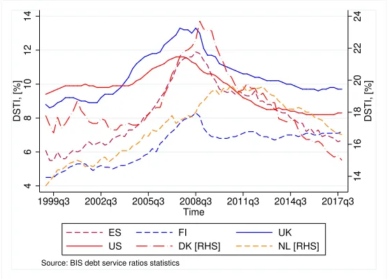
[image:16.612.167.446.385.585.2]The case of DSTI ratio is special because there is no precise information avail-able for its level neither in micro nor in aggregate data. However, an alternative is the BIS’s debt service ratios statistics database. This source provides in-ternationally consistent, country-specific quarterly data which ”should correctly capture how the [DSTI] in a particular country changes over time, even if it does not necessarily accurately measure its level relative to what one could ob-tain from the correct micro data” (Drehmann et al., 2015, p. 91). Although this is an aggregate measure and likely different from the bank-level one based on borrower basis as already recognized, in this study is assumed that the evo-lution of the two is roughly similar and thus the former can be used to provide an adequate approximation of the latter.
Figure 3 shows the evolution of DSTI ratio for households and NPISHs for a sample of EU countries and the US.
14
16
18
20
22
24
DSTI, [%]
4
6
8
10
12
14
DSTI, [%]
1999q3 2002q3 2005q3 2008q3 2011q3 2014q3 2017q3
Time
ES FI UK
US DK [RHS] NL [RHS]
Source: BIS debt service ratios statistics
Figure 3: Evolution of DSTI ratio for households and NPISHs in a sample of countries.
Figure 3 shows that the aggregate DSTI ratios in the plotted countries share
14
Eurostat dataset code:earn mw cur
15
a common evolution. A rapid growth roughly until the end of 2008, followed by a decline with diverse degrees of severity.
Apart from the UK for which there are available data on DSTI, the selec-tion of the remaining DSTI series to calibrate and match with the Estonian, Lithuanian and Slovenian historical macroeconomic scenario is based on the as-sumption that economic conditions in these countries resembled those in their larger European counterparts. Therefore, this should be reflected on an
ap-proximately comparable evolution of DSTI ratios.16 Data for the US are also
included because, as can be seen in Figure 3, its DSTI shares a similar pattern with that of several European economies.
The calibration procedure is described in detail in Appendix A and consists
of a grid-search to find which pair of{initial DSTI, DSTI path} minimizes the
distance between the artificial and actual series of consumption and credit.
3.2
Empirical validation
In the empirical validation of the model its output is examined under a baseline setup where all variables and their paths are set according to a country-specific, historical scenario. The ultimate goal is to test its ability to produce close to real-world patterns and thus establish confidence in its results and use for policy simulations.
It should be emphasized that the degree of similarity between the imple-mented country-specific scenario and the real-world one is of paramount impor-tance for the validation exercise. In that respect, the applied macroeconomic scenario for income and unemployment’s evolution can be regarded to repli-cate the realized one in a sufficient manner, even under the assumption of that evolution being uniform across income distribution as described in subsection 2.3.5. However, the results from the DSTI calibration procedure described in Appendix A indicate that only in two countries (SI and UK) the calibrated DSTIs can satisfactorily reproduce the historical evolution of consumer credit. This suggests that the identified DSTI paths for these two cases are, potentially, a decent match of the actual ones. Therefore, for the validation exercise and the subsequent simulation experiments where DSTI is evolving through time the focus will be only on these two countries (SI and UK). The validation results for the other cases are reported in Appendix B, while for the simulations where DSTI is held fixed at a certain value, every country scenario is considered.
Income distribution parameters and scenario related variables are initialized
according to the historical data as of January 200017 which is the chosen origin
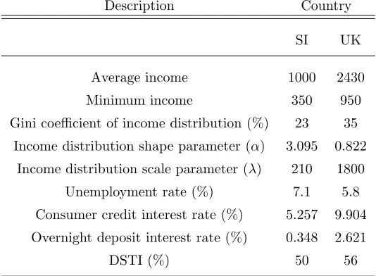
of the simulation. The initial setup of the simulations is provided in Table 2 and Table 7.
16
Of course country-specific factors are expected to affect the actual path of DSTI. Another source of divergence is the different evolution between consumer credit and mortgage DSTIs (see discussion in Appendix A for a detailed example). Thus, the final outcome depends on the degree of similarity between the actual and available data.
17
Table 2: Initial setup of the simulation for SI and UK.
Description Country
SI UK
Average income 1000 2430
Minimum income 350 950
Gini coefficient of income distribution (%) 23 35
Income distribution shape parameter (α) 3.095 0.822
Income distribution scale parameter (λ) 210 1800
Unemployment rate (%) 7.1 5.8
Consumer credit interest rate (%) 5.257 9.904
Overnight deposit interest rate (%) 0.348 2.621
DSTI (%) 50 56
After a burn-in period ofN = 170 time steps, the country-specific historical
[image:18.612.143.469.455.568.2]scenario is input to the model. A description of the series used and their time periods is provided in Table 3 and Table 8.
Table 3: The range of the variables used in SI and UK historical scenarios.
Variable SI UK
Wages & salaries 2000q1 - 2018q1 2000q1 - 2018q1
Unemployment rate 2000m1 - 2018m3 2000m1 - 2018m3
Consumer credit interest rate 2005m5 - 2018m3 2004m1 - 2018m3
Overnight deposit interest rate 2005m5 - 2018m3 2004m1 - 2018m3
DSTI path US UK
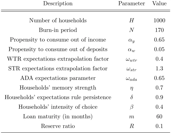
Besides scenario and initialization data which are country-specific, a set of parameters associated with agents’ behaviour as well as to the model’s setup is fixed across simulations and reported in Table 4.
Table 4: Fixed parameter values.
Description Parameter Value
Number of households H 1000
Burn-in period N 170
Propensity to consume out of income αy 0.65
Propensity to consume out of deposits αw 0.05
WTR expectations extrapolation factor ωwtr 0.4
STR expectations extrapolation factor ωstr 1.3
ADA expectations parameter ωada 0.65
Households’ memory strength η 0.7
Households’ expectations rule persistence δ 0.9
Households’ intensity of choice β 0.4
Loan maturity (in months) m 60
Reserve ratio R 0.1
Propensities to consume (αyandαw) are set to values commonly used by the
literature (Godley and Lavoie, 2016; Assenza et al., 2015; Meijers et al., 2018, among others), while the HSM-related parameters are specified according to the figures identified by Anufriev and Hommes (2012a,b). The unemployment dole, coinciding with the subsistence consumption level, is assumed to be 80% of minimum income at each step of the simulation.
3.2.1 Validation with the Slovenian scenario
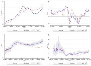
The results for the Slovenian scenario, plotted in Figure 4, exhibit a decent match between artificial and historical data.
.8
.9
1
1.1
1.2
C t
/C
mean
2000q1 2003q1 2006q1 2009q1 2012q1 2015q1 2018q1
Time
Historical Simulation P25/P75
−5
0
5
10
%
∆yoy
2001q3 2005q3 2009q3 2013q3 2017q3
Time
Historical Simulation P25/P75
0
.5
1
1.5
2
L t
/L
mean
2004m1 2006m1 2008m1 2010m1 2012m1 2014m1 2016m1 2018m1 Time
Historical Simulation P25/P75
−20
0
20
40
60
80
%
∆yoy Lt
2004m1 2006m1 2008m1 2010m1 2012m1 2014m1 2016m1 2018m1
Time
[image:20.612.134.481.178.430.2]Historical Simulation P25/P75
Figure 4: Baseline simulation results for the SI-specific scenario.
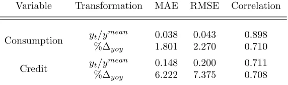
Firstly, simulated consumption displays a remarkable degree of similarity in terms of distance and synchronicity with the historical series. Moreover, simulated consumer credit data exhibit a high degree of resemblance to the evolution and magnitude of the historical series. This is indicated by the fact that, in addition to the median simulation being fairly close to the actual data, the latter lie between the first and third quartile (P25/P75) bands of the former for a large part of the simulation horizon. The divergence originates in 2013 when the artificial series begin to rise (Figure 4, bottom left pane), while the historical ones continue to decline up to 2016. This is associated with the financial difficulties faced by the domestic banking system at the time (Bank of Slovenia, 2013) resulting in a negative growth of consumer loans which only ”moved into positive territory after six years [in 2016].” (Bank of Slovenia, 2016, p.44). Therefore, during this period, the assumed DSTI path used in the model is most likely more benign from what occurred in reality. However, after early 2017 the two series resume their co-movement indicating that from then on the assumed DSTI path is again an adequate approximation of the actual one.
informa-tion on the findings of Figure 4.
Table 5: Distance and similarity measures between simulated and historical data for SI.
Variable Transformation MAE RMSE Correlation
Consumption yt/y
mean 0.038 0.043 0.898
%∆yoy 1.801 2.270 0.710
Credit yt/y
mean 0.148 0.200 0.711
%∆yoy 6.222 7.375 0.708
The distance between artificial and observed consumption is around 2% in growth rates and about 4% in rescaled levels. At the same time, correlation is high and ranges from 70% to almost 90%. An important finding is that simulated consumer credit growth exhibits an average distance of 6% to 7% from the historical one while correlation remains at sufficiently high levels of about 70%.
3.2.2 Validation with the UK scenario
The next scenario considered for validation purposes is the UK-specific one.
Data for DSTI’s path are available for this country18, which results in the closest
emulation of consumer credit evolution generated by the model. The output is presented in Figure 5.
18
.8
.9
1
1.1
1.2
C t
/C
mean
2000q1 2003q1 2006q1 2009q1 2012q1 2015q1 2018q1
Time
Historical Simulation P25/P75
−5
0
5
%
∆yoy
2001q3 2005q3 2009q3 2013q3 2017q3
Time
Historical Simulation P25/P75
0
.5
1
1.5
2
L t
/L
mean
2002m1 2004m1 2006m1 2008m1 2010m1 2012m1 2014m1 2016m1 2018m1 Time
Historical Simulation P25/P75
−20
0
20
40
60
%
∆yoy Lt
2004m1 2006m1 2008m1 2010m1 2012m1 2014m1 2016m1 2018m1 Time
[image:22.612.135.482.123.376.2]Historical Simulation P25/P75
Figure 5: Baseline simulation results for the UK-specific scenario.
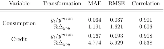
As seen in Figure 5, apart from simulated consumption series which show the, common among all scenarios (see also results in Appendix B), noteworthy similarity to the actual ones, simulated consumer credit exhibits the highest de-gree of closeness to the historical series from all scenarios examined. First and third quartile bands envelop the actual data for almost the entire simulation horizon both in levels and in growth rates. An obvious exception is observed to-wards the end of the simulation, approximately after early 2016, when simulated series begin to flatten and growth rates to decline whereas the actual ones show an upward trend (with the respective growth rates being on positive ground). It should be mentioned that to avoid distortions related to very low figures in the beginning of the simulation horizon, observations prior to December 2002 are discarded from the analysis.
Table 6: Distance and similarity measures between simulated and historical data for UK.
Variable Transformation MAE RMSE Correlation
Consumption yt/y
mean 0.034 0.037 0.901
%∆yoy 1.191 1.621 0.606
Credit yt/y
mean 0.167 0.193 0.918
%∆yoy 4.774 5.929 0.538
As expected, the results in Table 6 are the best among all scenarios exam-ined. Simulated consumption displays the minimum distance and high correla-tion with actual data. Despite the fact that correlacorrela-tion between artificial and observed growth rates is relatively low compared to the other cases, it is still at the satisfactory level of about 60% while at the same time both MAE and RMSE are below 2%. Results on consumer credit show a similar pattern; an average correlation accompanied by the lowest distance in growth rates and the highest correlation with comparable distance measures in rescaled levels.
Overall the validation exercise revealed three common patterns among all scenarios; first, there is a remarkably good fit between artificial and actual data on consumption. This indicates that the implemented consumption rule com-bined with data on disposable income can provide an appropriate approxima-tion of aggregate consumpapproxima-tion. Second, Q1/Q3 bands around median simulated consumption are very narrow. Since the stochastic element associated with con-sumption comes from consumer credit, this indicates that the latter is a small fraction of consumption. Finally, simulated consumer credit is adequately close to the observed data where available data for DSTI are a good approximation of the realized series. This enhances trust in the validity of the model to ap-propriately capture the underlying credit supply mechanism and reproduce its dynamics once reliable data are used as input.
3.3
The role of expectations on credit demand
A key element of the ABM under development is the implementation of the HSM for agents’ expectations. The vast majority of macroeconomic ABMs is mainly endowing their agents with a single or, in some cases, two expectations
heuristics. The most frequently used choices include naive expectations (ye
t =
yt−1), an adaptive rule similar to that in Equation 4 or some form of
trend-extrapolative rule analogous to Equation 2. Other choices range from regressive techniques to rational expectations. The interested reader is referred to the excellent work of Franke and Westerhoff (2017) and references therein for a survey of modelling of animal spirits.
the HSM is used, is by Dosi et al. (2017) where the authors find that expectations do not have a large effect on the dynamics of the economy.
However, credit demand in the present model depends heavily on income expectations and is essentially determined by households’ forecast errors; op-timistic households whose actual income is less than expected will likely ask for credit; on the contrary, pessimistic households will consume less, save more and deleverage. Therefore, given the central role that expectations play in the model, their effect on credit dynamics will be further examined.
All initialization parameters are set as reported in Table 2 with the exception of DSTI which is kept fixed at 100% over the whole simulation. This large value is chosen in order to enable the bank to accommodate practically any credit request, even if the associated monthly payment equals the borrower’s income. Using each individual expectations heuristic alone, plus all four of them with the switching mechanism of the HSM, the evolution of credit for each macroeconomic scenario is examined and presented in Figure 6.
0 500000 1000000 Lt 2000m1 2002m1 2004m1 2006m1 2008m1 2010m1 2012m1 2014m1 2016m1 2018m1 Time
WTR STR ADA
LAA HSM EE 0 500000 1000000 1500000 Lt 2000m1 2002m1 2004m1 2006m1 2008m1 2010m1 2012m1 2014m1 2016m1 2018m1 Time
WTR STR ADA
LAA HSM LT 0 1000000 2000000 Lt 2000m1 2002m1 2004m1 2006m1 2008m1 2010m1 2012m1 2014m1 2016m1 2018m1 Time
WTR STR ADA
LAA HSM SI 0 1000000 2000000 Lt 2000m1 2002m1 2004m1 2006m1 2008m1 2010m1 2012m1 2014m1 2016m1 2018m1 Time
WTR STR ADA
LAA HSM
[image:24.612.134.481.313.568.2]UK
Figure 6: Outstanding credit evolution for different expectations heuristics.
line), being a trend extrapolation one, also generates increased credit demand
but not as high as the STR rule. Interestingly, mean19 outstanding credit is
absent in the cases of WTR and ADA rules. This indicates that under these rules income expectations are very close to the realized figures or they are down-wards biased. In the former case, the desired consumption demand from any small, optimistic income forecast can be met by deposit withdrawal. In case expectations are downwards biased, the actual income suffices to satisfy desired consumption therefore credit is not needed. Finally, the HSM being a changing mixture of all four rules, results in levels of credit which are influenced by the dominating heuristic and in any case lie between the polar cases of STR and
WTR (or ADA). This is more evident in the case of the UK scenario20 where
the simulation indicates that the LAA rule is heavily dominating, hence the results of the HSM are very close to the LAA’s.
The differential effect of expectations heuristics on the level of credit raises the question whether this could also affect the size and evolution of non-performing
loans ratio (NPL21). The results for NPLs are extracted from the previous
sim-ulations for the heuristics that did lead to credit growth (STR, LAA and the HSM) and are plotted in Figure 7.
19
Results are the same even up to the 75th
percentile of all simulation runs.
20
Including initialization parameters. This is due to the fact that forecast errors for variables with sizable values in absolute terms (such as the average and minimum income related to the UK scenario) will be also large, thus influencing heuristic selection.
21
0
10
20
NPL
t
, [%]
2000m1
2002m12004m12006m12008m12010m12012m12014m12016m12018m1 Time
STR LAA HSM
EE
0
10
20
NPL
t
, [%]
2000m1
2002m12004m12006m12008m12010m12012m12014m12016m12018m1 Time
STR LAA HSM
LT
0
5
10
NPL
t
, [%]
2000m1
2002m12004m12006m12008m12010m12012m12014m12016m12018m1 Time
STR LAA HSM
SI
0
2
4
6
NPL
t
, [%]
2000m1
2002m12004m12006m12008m12010m12012m12014m12016m12018m1
Time
STR LAA HSM
[image:26.612.134.482.123.376.2]UK
Figure 7: Non-performing loans (≥180 days past due) ratio evolution for
dif-ferent expectations heuristics.
Figure 7 shows that average NPL evolution and size is almost identical among heuristics in three out of four cases. The exception is the UK-specific scenario where under the LAA rule average NPLs start to rise with an approximate 2-year lag compared to the STR rule and the HSM. Apart from this discrepancy, the size as well as the evolution is comparable among all expectations heuristics. The previous analysis suggests that expectations heuristics have differential and significant impact on the levels of provided credit, with some even resulting in its complete absence. Nevertheless, differences among those which do result in credit demand are not substantial neither in its growth rate nor in the size and evolution of NPLs. Consequently, taking also into account the experimental evidence by the respective literature, the HSM will be used throughout this study.
3.4
Inequality, credit supply and macro-financial
develop-ments
second fixes DSTI at certain values throughout the simulation and analyzes the impact of different initial levels of income inequality. The results from the experiments are discussed below.
3.4.1 Evolving DSTI
In the first experiment is examined the effect of initial income inequality on con-sumption, credit and NPLs. The simulation is executed with the only difference from the baseline settings being in the initial level of income inequality. For various income distribution Gini coefficients spanning from approximately 22% to about 38% the model is run 100 times using two of the scenarios examined (SI
and UK) and the results over the whole simulation horizon are averaged22 and
reported in Figure 8 to Figure 10. To facilitate comparison, results are bench-marked against the figure at the highest level of inequality. Hence, the vertical
axis corresponds23
to %∆y∗
λ = 100(
yλ
y∗ −1), where y ={C, L},yλ the value of
variabley at scaleλandy∗is the benchmark value of variabley. The two
hori-zontal axes in the respective graphs denote the initial scale parameter,λ, of the
Γ(α,1/λ) income distribution (bottom) or, equivalently, the corresponding Gini
coefficient (top). In addition, the regression lines %∆y∗
λ=βy·Gini+constanty
are drawn and the estimatedβy coefficients with the corresponding statistical
significance levels are reported.
The results for consumption are presented in Figure 8.
−.5
0
.5
1
1.5
%
∆
Cλ
*, [%]
.223 .261 .291 .314 .334 .352 .367 .381 Gini coefficient
200 300 400 500 600 700 800 900
λ
***/**/* indicates significance at the 1/5/10 percent level
β = −7.386***
SI
−1
−.5
0
.5
%
∆
Cλ *, [%]
.229.243.256.267.279.287.297.305.314.320.328.336.341.346.352.357.363.369 Gini coefficient
600 700 800 900 1000 1100 1200 1300 1400 1500 1600 1700 1800 1900 2000 2100 2200 2300
λ
***/**/* indicates significance at the 1/5/10 percent level
β = −4.654***
[image:27.612.137.482.394.522.2]UK
Figure 8: The effect of income inequality on average consumption. The red×
denotes the benchmark value.
Figure 8 exhibits a clear, negative relationship between income inequality and average consumption for both scenarios. This is also manifested in the sta-tistically significant coefficients of the respective regression lines which indicate that a 1% decrease in Gini coefficient of income distribution results in an ap-proximate 0.04% to 0.07% increase in average consumption, depending on the
22
Specifically, it’s the whole period average of the average over the 100 runs.
23
In the case of NPLs, the latter being already expressed as a ratio, the distance from the
scenario examined. The sign of the relationship is as expected. When income is more equally distributed, then a larger number of households have more funds available thus resulting in higher levels of consumption. On the contrary, when income is more concentrated, consumption cannot be supported by the few at the top of the distribution and therefore settles in lower average values. In the next subsection is examined whether considerably looser credit supply can mit-igate the detrimental effect of inequality on consumption. Moving to consumer credit, Figure 9 reveals an interesting pattern.
−20
0
20
40
60
%
∆
Lλ *, [%]
.223 .261 .291 .314 .334 .352 .367 .381
Gini coefficient
200 300 400 500 600 700 800 900
λ
***/**/* indicates significance at the 1/5/10 percent level
β = −242.41***
SI
−20
0
20
40
60
%
∆
Lλ *, [%]
.229.243.256.267.279.287.297.305.314.320.328.336.341.346.352.357.363.369 Gini coefficient
600 700 800 900
1000 1100 1200 1300 1400 1500 1600 1700 1800 1900 2000 2100 2200 2300
λ
***/**/* indicates significance at the 1/5/10 percent level
β = −246.611***
[image:28.612.134.480.231.358.2]UK
Figure 9: The effect of income inequality on average consumer credit. The red
×denotes the benchmark value.
As seen in Figure 9, income inequality does affect the average volume of consumer credit. In particular, a 1% increase in the former (more precisely in income distribution’s initial Gini coefficient) results in an approximate decrease of the latter by 2.4% as suggested by the respective regressions.
affect the results, obscuring the potential underlying causal relationship. Even in the best case where household credit comprising of mortgages and consumer loans is considered, the different dynamics of the two components might have substantial impact on the results obtained and their interpretation. Indeed, data from Jord`a et al. (2015) show that the trends and levels of the two types of
credit are noticeably different in 17 countries24
, resulting in a 20% difference as a share of GDP around 2012. The possibly different mechanism associated with housing credit as opposed to consumer credit might imply a different explana-tion for credit growth than the need of low income households supporting their living standards (Bazillier and H´ericourt, 2014). In fact, Coibion et al. (2014) using household level data reject the ”keeping up with the Joneses” hypothesis, i.e. the demand-side explanation of credit growth and find a negative relation between inequality and household debt.
The pattern observed in Figure 9 is also associated with the supply-side of credit. The mechanism works through the adequately high income being held by a large number of households. This configuration results in more credit being considered as affordable by the banking sector (i.e. supported by the
potential borrowers’ income) for a given DSTI25 and therefore being granted
once it is asked for, assuming that demand remains roughly the same under
different inequality regimes26
. Another key driver of this result is households’ assumed consumption function in Equation 1. Since habit formation or com-parison with some external reference level are not explicitly considered, desired consumption -and by extension consumer credit demand- is driven by income expectations. Nevertheless, once credit demand is expressed it is for the bank to decide how much to lend according to its DSTI level. Hence, households exceeding the bank’s risk tolerance will be rationed and credit supply effectively limited. Finally, results for NPLs are shown in Figure 10.
−1.5
−1
−.5
0
.5
∆
NPL
λ
*, [%]
.223 .261 .291 .314 .334 .352 .367 .381
Gini coefficient
200 300 400 500 600 700 800 900
λ
***/**/* indicates significance at the 1/5/10 percent level
β = −.766
SI
−1.5
−1
−.5
0
.5
∆
NPL
λ
*, [%]
.229.243.256.267.279.287.297.305.314.320.328.336.341.346.352.357.363.369 Gini coefficient
600 700 800 900 1000 1100 1200 1300 1400 1500 1600 1700 1800 1900 2000 2100 2200 2300
λ
***/**/* indicates significance at the 1/5/10 percent level
β = 3.568*
[image:29.612.131.480.460.585.2]UK
Figure 10: The effect of income inequality on average NPLs. The red×denotes
the benchmark value.
24
Especially in the period after early 2000s, which is the focus of the present study.
25
And other supply-side related properties such as loan interest rates and maturities.
26
Figure 10 suggests that the relationship between income inequality and av-erage NPLs is weak at best or possibly non-existent. In the UK-specific scenario (right graph in Figure 10), higher inequality is associated with higher NPLs, al-though the magnitude of the relationship is small and its statistical significance low. On the contrary, in the case of the SI-specific scenario NPLs seem to be independent from the level of income inequality, something which is reflected on the statistically insignificant (i.e. indistinguishable from zero) slope of the respective regression line. The main reason behind this result is the volume of consumer credit.
The volume of credit provided is primarily controlled by the interaction between the expectations-based demand and the DSTI-constrained supply. In general, the amount of consumer credit asked is small since income expectations are never that extraordinarily far from the realized values to render households’ available financial resources inadequate to cover an important part of desired
consumption. In addition, DSTI limits themaximum monthly loan installment
of an indebted household at the level of 50% to 60% of its income, depending on the scenario applied (see Table 3). Finally, the debt assumed by a household stochastically ranges between the demanded and the maximum amount offered (see Equation 11). Thus, it is more probable that it will be lower than the upper value permitted by DSTI at any point in time. The interplay of these mechanisms results in the respective monthly installments being a small fraction of households’ income, hence facilitating loan servicing even if income declines considerably. Therefore, the main driver of NPLs is unemployment, the latter being the reason for substantial income reduction, rendering debt unserviceable. The stochastic, income-independent nature of unemployment shocks results in NPLs being unconnected with the levels of inequality. It is possible that differential unemployment growth across the distribution of income might influ-ence the result depending on the direction and the degree of unemployment’s impact. In case unemployment rises more among households at the bottom of income distribution than among those at the top, a stronger link between NPLs and inequality -conditional on the severity of this increase- could be expected. On the contrary, if the impact of unemployment is stronger among households at the top of income distribution -who, in general, do not resort to borrowing to meet their consumption needs- the relationship between NPLs and inequality is expected to be weak at best. The scarcity of exact data on unemployment’s evolution by income percentile does not allow for the development of a more
accurate historical scenario27
, thus the baseline assumption of a uniform effect of unemployment will be applied, bearing in mind the caveats discussed above. It should be reminded that NPLs are defined as the share of loans past due 6 months to total loans. Obviously, if instead of the ratio is considered the level
27
of non-performing loans the sign of the relationship is clearly negative. Lower income inequality and its associated larger volumes of credit are more likely to result in higher amounts of non-performing obligations. In that respect, NPLs expressed as ratio is a more meaningful metric.
3.4.2 Fixed DSTI
In this experiment, besides the effect of initial income inequality, is also studied the effect of different DSTIs on consumption, credit and NPLs. In particular, DSTI ranges from 50% up to 80% and remains fixed throughout the simulation. Moreover, for each DSTI level the model is run 100 times with different initial income distribution Gini coefficients which span from about 22% to 38%. The rest of the macroeconomic scenario remains at its baseline setup.
The average of every variable over the whole simulation per {DSTI, initial
Gini coefficient} pair is plotted in Figure 11 to Figure 13. The benchmark
against which the comparison is made, as well as the horizontal axes follow the same conventions as in the previous experiment. The vertical axis represents the various DSTI levels while the colour of each cell indicates their distance from the associated zero-level.
X .5 .55 .6 .65 .7 .75 .8 DSTI
.243 .280 .307 .331 .350 .366 .381
Gini coefficient
50 75
100 125 150 175 200
λ 0.0 1.0 2.0 3.0 4.0 % ∆ C λ *, [%] EE X .5 .55 .6 .65 .7 .75 .8 DSTI
.235 .267 .290 .310 .325 .340 .352 .363 .373
Gini coefficient
50 75
100 125 150 175 200 225 250
λ 0.0 1.0 2.0 3.0 4.0 % ∆ Cλ *, [%] LT X .5 .55 .6 .65 .7 .75 .8 DSTI
.223 .244 .261 .276 .290 .303 .315 .325 .335 .343 .353 Gini coefficient
200 250 300 350 400 450 500 550 600 650 700
λ −0.5 0.0 0.5 1.0 1.5 % ∆ Cλ *, [%] SI X .5 .55 .6 .65 .7 .75 .8 DSTI
.221 .243 .262 .278 .292 .305 .317 .328 .337 .347 Gini coefficient
550 700 850
1000 1150 1300 1450 1600 1750 1900
[image:31.612.134.477.353.605.2]λ 0.0 0.2 0.4 0.6 0.8 1.0 % ∆ Cλ *, [%] UK
Figure 11: Average consumption per DSTI and initial income inequality level.
The red×denotes the benchmark value.
Results in Figure 11 display an interesting pattern. For low levels of income
than the benchmark even for low levels of DSTI. This difference is more sizable in economies with lower absolute levels of minimum and average income, fluctu-ating around 4% as shown in the first row of Figure 11. As these distributional parameters increase, the magnitude of the effect declines to 1% - 1.5% although the general pattern remains the same. As one moves to higher levels of inequal-ity, consumption does not seem to be substantially supported by looser credit supply and settles to lower values. Finally, at the high inequality regions of the graphs consumption is evidently lower for any DSTI level as indicated by the more frequent cold-coloured patches in Figure 11.
Results for consumer credit are presented in Figure 12 and display a rather expected structure. X .5 .55 .6 .65 .7 .75 .8 DSTI
.243 .280 .307 .331 .350 .366 .381
Gini coefficient
50 75
100 125 150 175 200
λ 0.0 50.0 100.0 150.0 200.0 250.0 % ∆ Lλ *, [%] EE X .5 .55 .6 .65 .7 .75 .8 DSTI
.235 .267 .290 .310 .325 .340 .352 .363 .373
Gini coefficient
50 75
100 125 150 175 200 225 250
λ 0.0 100.0 200.0 300.0 % ∆ Lλ *, [%] LT X .5 .55 .6 .65 .7 .75 .8 DSTI
.223 .244 .261 .276 .290 .303 .315 .325 .335 .343 .353 Gini coefficient
200 250 300 350 400 450 500 550 600 650 700
λ 0.0 50.0 100.0 150.0 200.0 250.0 % ∆ Lλ *, [%] SI X .5 .55 .6 .65 .7 .75 .8 DSTI
.221 .243 .262 .278 .292 .305 .317 .328 .337 .347 Gini coefficient
550 700 850
1000 1150 1300 1450 1600 1750 1900
[image:32.612.135.477.265.517.2]λ 0.0 100.0 200.0 300.0 400.0 % ∆ Lλ *, [%] UK
Figure 12: Average consumer credit per DSTI and initial income inequality
level. The red×denotes the benchmark value.
In general, for any level of initial income inequality, an increase in DSTI levels is followed by an increase in the average volume of consumer credit. However, results indicate that income inequality does affect credit provision, with the sign of the relationship corroborating the findings of the previous experiment. For a given DSTI, average consumer credit is higher for smaller Gini coefficients and drops as the latter increases. It should be noted here that the considerably wide range of results is due to the small value of the benchmark, generated under the minimum DSTI examined.
X .5 .55 .6 .65 .7 .75 .8 DSTI
.243 .280 .307 .331 .350 .366 .381
Gini coefficient
50 75 100 125 150 175 200
λ −0.5 0.0 0.5 1.0 1.5 ∆ NPL λ *, [%] EE X .5 .55 .6 .65 .7 .75 .8 DSTI
.235 .267 .290 .310 .325 .340 .352 .363 .373
Gini coefficient
50 75 100 125 150 175 200 225 250
λ −0.5 0.0 0.5 1.0 1.5 2.0 ∆ NPL λ *, [%] LT X .5 .55 .6 .65 .7 .75 .8 DSTI
.223 .244 .261 .276 .290 .303 .315 .325 .335 .343 .353 Gini coefficient
200 250 300 350 400 450 500 550 600 650 700
λ 0.0 1.0 2.0 3.0 4.0 ∆ NPL λ *, [%] SI X .5 .55 .6 .65 .7 .75 .8 DSTI
.221 .243 .262 .278 .292 .305 .317 .328 .337 .347 Gini coefficient
550 700 850 1000 1150 1300 1450 1600 1750 1900
[image:33.612.133.477.120.372.2]λ −1.0 0.0 1.0 2.0 3.0 ∆ NPL λ *, [%] UK
Figure 13: Average NPLs per DSTI and initial income inequality level. The red
×denotes the benchmark value.
In line with the results of the experiment with evolving DSTI, Figure 13 suggests that there is no apparent link between the average level of NPLs and income inequality for any DSTI level. Cold and warm-coloured patches are alternating with no clear structure emerging within the range of DSTIs and Gini coefficients examined.
4
Conclusions
This study examined the effect of income inequality on consumption, credit and non-performing loans by the means of a simple, data-driven agent-based model. For its development are used standard elements from the respective macroe-conomic ABM literature, augmented with a heuristics switching model based on the findings from experimental studies on expectations formation. Overall, its structure is kept simple by replacing the actions of and interactions among some agents with the historical evolution of the associated series. This simplic-ity allows the model’s output to be a markedly close replication of the actual data when input is accurate enough.
be readily used to provide scenario analyses examining the impact of macropru-dential regulations (e.g. DSTI or consumer loan maturity limits) on consump-tion and credit growth, condiconsump-tional on income and unemployment’s evoluconsump-tion.
The experimental simulations performed with the model indicate that, in the long run, income inequality is negatively associated with both consumption and the volume of consumer credit. The former result is as expected. A more equal distribution of income implies that a larger number of households have more purchasing power available thus being able to maintain higher consumption lev-els. The latter result corroborates the findings of recent empirical studies which find a negative relationship between inequality and household debt. An inter-esting result is that the ratio of non-performing obligations as a share of total consumer credit seems to be independent of inequality. This is the outcome of the interplay between two mechanisms governing the volume of consumer credit; an expectations-based demand and a DSTI-constrained supply. These mecha-nisms result in serviceable debt levels even under significant income decreases for any inequality level. Obviously, this result should not be linked with the large volume of mortgages observed in many countries since the early 2000s and the associated non-performing obligations which cannot be studied under the current implementation of the model.
Future research aims at extending the model in several dimensions, while maintaining its close link with the actual data. A first step will be to include agents which in the current version are assumed to be exogenous such as firms or a more elaborate banking sector reacting to central bank’s actions. Equipping the model with more active agents will also permit a more detailed description of various markets such as the labour market or the incorporation of additional ones such as the housing market. These extensions will allow to study the effect of implementing and the interactions among various economic policies thus assisting policy makers in supporting and promoting societies’ well-being.
References
Allen, T. W. and Carroll, C. D. (2001). Individual learning about consumption. Macroeconomic Dynamics, 5(02):255–271.
Amaral, P. (2017). Monetary policy and inequality. Federal Reserve Bank of
Cleveland Economic Commentary 2017-01.
Ampudia, M., Georgarakos, D., Slacalek, J., Tristani, O., Vermeulen, P., and
Violante, G. (2018). Monetary policy and household inequality.ECB Working
Paper, No. 2170.
Anufriev, M. and Hommes, C. (2012a). Evolution of market heuristics. The
Knowledge Engineering Review, 27(2):255–271.
Anufriev, M. and Hommes, C. (2012b). Evolutionary selection of individual
expectations and aggregate outcomes in asset pricing experiments.American