ISSN Online: 2160-8849 ISSN Print: 2160-8830
DOI: 10.4236/ajor.2017.76027 Nov. 27, 2017 356 American Journal of Operations Research
A Review of Activity Time Distributions in
Risk Analysis
Enobong Francis Udoumoh
1, Daniel W. Ebong
21Department of Mathematics/Statistics/Computer Science, University of Agriculture, Makurdi, Nigeria 2Department of Mathematics and Statistics, University of Port Harcourt, Port Harcourt, Nigeria
Abstract
Project Evaluation and Review Technique (PERT) alongside recent modifica-tions is a popular and useful tool in project risk analysis. Over the past seven decades, there have been some modifications in PERT owing to the shift from beta distributed activity times to other activity time distributions. This paper presents a review of activity time distributions in risk analysis as found in li-terature up to date.
Keywords
PERT, Project Network, Activity Duration, Probability Distributions
1. Introduction
Project Evaluation and Review Technique (PERT) is widely used by project managers and practitioners as the probabilistic form of the Critical Path Method (CPM). The PERT method is not only useful for the estimation of project com-pletion times but it is also workable and cost-effective for management of projects [1]. PERT has become of interest to management practitioners because of its simplicity, and flexibility to accommodate stochastic activity times. PERT was invented in 1958 for the POLARIS Missile Program by the Program Evalua-tion branch of the Special projects Office of US Navy [2]. Malcom’s PERT net-work, henceforth referred to as classical PERT netnet-work, assumes that all activi-ties are independent random variables, having approximately beta distributions parameterized by three times estimates: the optimistic time a, the pessimistic time b, and the most likely time m. The expected time of each activity is ob-tained using the formula
(
a+4m b+)
6 and standard deviation presented as one sixth of the range of the distribution resulting to(
b a−)
2 36 as theva-How to cite this paper: Udoumoh, E.F. and Ebong, D.W. (2017) A Review of Ac-tivity Time Distributions in Risk Analysis. American Journal of Operations Research, 7, 356-371.
https://doi.org/10.4236/ajor.2017.76027
Received: October 22, 2017 Accepted: November 24, 2017 Published: November 27, 2017
Copyright © 2017 by authors and Scientific Research Publishing Inc. This work is licensed under the Creative Commons Attribution International License (CC BY 4.0).
DOI: 10.4236/ajor.2017.76027 357 American Journal of Operations Research riance. The critical path is then computed as the longest path. With the belief that the network is large enough, the central limit theorem is applied to estimate the project completion time. For detail application of PERT, interested readers are referred to [1] [2].
Although it is well accepted that the classical PERT gives useful estimates, its assumption introduces some potential sources of bias which results in the unde-restimation of project completion time [3] [4] [5]. Sources of PERT bias as do-cumented in literature include: the misspecification of the activity time distribu-tion, the method of computing critical path by ignoring the near critical activi-ties, and the possible violation of the normality assumption during the estima-tion of project compleestima-tion time. There exist a sharp divide among researchers with respect to the need for introduction of new activity duration distributions in PERT. For instance, earlier works by Clark [6], Kamburowski [7] supported the use of Beta distribution. Recently, Hajdu and Bokor [8] argued still in sup-port of the Beta distribution. They considered the following “hypothetical” judgemental estimates: 60-optimistic, 100-most likely, and 150-pessimistic whose skewness coefficient is only 0.09826. The beta distribution defined by this coeffi-cient of skewness is the one that approximates the normal distribution which is also supported by PERT-Beta approximation. Hence, there is no doubt about their conclusion. In spite of this, the graphical results that compared the PERT-Beta, triangular and uniform distributions still showed some obvious variations. It is possible that a set of data with much longer tail would have yielded worse re-sults. Moreover, a comparison done with many more activity time distributions would have given more in-depth revelations. On the other hand, some research-ers opine that the adoption of Beta distribution was intuitive as there was no empirical evidence for its usage. For instance, it has been demonstrated by Mac-Crimmon and Ryavec [3] that the error for classical PERT calculated mean and standard deviation could be up to 33% and 16% respectively. This point was buttressed by Williams [9] using simulation and graphical approaches to dem-onstrate the extent of discrepancies that exist between the beta and triangular distributions in the estimation of activity time parameters. Hahn and Martín [10] support the use of a more robust distribution that can accommodate outly-ing events. An undisputed observation in project management is that most ac-tivity time distributions are right skewed [11] [12] [13].
The importance of probability distributions in PERT cannot be overempha-sized as both the simulation and analytical approaches assume probability dis-tributions for activity durations a priori or a posteriori [5] [14] [15]. Conse-quently, researchers have suggested various activity duration distributions for the analyses of project networks. Unfortunately, most basic texts in operations research and project management present only PERT-beta distribution without any mention of other activity time distributions.
DOI:10.4236/ajor.2017.76027 358 American Journal of Operations Research of PERT-Beta approach are also presented. We further highlight the various methods adopted for parameter estimation based on these distributions.
2. Activity Time Distributions in Literature
1) The Beta DistributionThe originators of classical PERT [2] assumed that project activity time fol-lows the generalized beta distribution with probability density function
( )
( ) ( )
(
)
(
) (
)
(
)
1 1
1 ; , , 0
x a b x
f x a x b
b a α β α β α β α β α β − − + −
Γ + − −
= < < >
Γ Γ −
where
α
and β are the shape parameters, Γ( )
. is the gamma function. The mean, variance and skewness are respectively given as(
)
x a b a
α µ α β = + − + ,
(
)
(
) (
)
2 2 2 1x b a
αβ σ
α β α β
= − + + + and
(
)
(
)
1 2 1 2 β α α β γα β αβ
− + +
=
+ +
In classical PERT, the mean and variance were estimated to be ˆ 4 6
x a m b
µ = + +
and
(
)
2 2 ˆ 36 x b a
σ = − . A study by Farnum and Stanton [16] revealed that the mean
of the beta distribution in classical PERT is appropriate within some range of modal values, namely, a+0.13
(
b a−)
< < −m b 0.13(
b a−)
. This means that the estimate performs poorly outside this interval. This can either happen when the most likely estimate, m, is chosen to be very close to the two extreme values, aand b, (less than 13% of the range from either a or b). In other words the classic-al PERT estimate fails when activity time distributions are heavily tailed. More-over, previous works reveal that the classical PERT assumptions of the mean and variance restrict us to only three members of the beta family, namely, 1)
4
α β= = ; 2) α = −3 2, β= +3 2; 3) α = +3 2, β = −3 2. In which case the skewness will be 0, 1
2 and 1 2
− respectively [17] [18] [19]. This
restriction led to various modifications on the classical PERT to accommodate more members of the beta family. We will discuss some of these modifications. Most of these modifications are based on the adjustments of the parameters of beta distribution.
Gollenko-Ginzburg [20] worked on the improvement of the classical PERT estimates based on only two subjective estimates the pessimistic 1) and optimis-tic 2) times. He posited that analysis of many project networks with lengthy pe-riods reveals that the most likely activity time is practically useless. He pointed out that its relative location in time interval
[ ]
a b, is usually close to the point2 3
a b
m= + . Given the density function
( )
(
Γ(
) (
2)
) (
)
( 1)1
Γ 1 Γ 1
x
p m p
p q
f x x x
p q
− + +
= −
DOI: 10.4236/ajor.2017.76027 359 American Journal of Operations Research (mx = mode of x) which was obtained after a re-parametisation of the standard
beta distribution, with additional assumption that p q Z+ ≅ (constant). The following results 2 9 2
13
y a m b
µ = + + and
(
)
2 22 22 81 81
1268 y
b a m a m a b a b a
σ = − + − − −
− −
were obtained for the estimation
of the mean and variance of activity distribution. He showed that these formulae provide better results as compared to the classical pert formulae when the esti-mated mode is located in the tails of the distribution. These formulae were fur-ther reduced to µy=0.2 3
(
a+2b)
and 2 0.04(
)
2y b a
σ = − on the basis of the earlier assumption of the mode, 2
3
a b+
≅ . A similar modification was carried
out by Shankar and Sireesha [21] on the classical PERT. The approximation was achieved by their so called generalization of the assumptions on the parameters of the classical PERT method. Given the density function,
( )
(
Γ(
) (
2)
) (
)
( 1)1
Γ 1 Γ 1
x
p m p
p q
f x x x
p q
− + +
= −
+ + with the relation p q K+ ≅ (constant). Also, substituting p+1 and q+1 for p and q respectively they obtained the
results 17 5
27x
x m
µ = + and 2
(
17 10 27 17)(
)
2300
x x
x
m m
σ = + − which give
5 17 5
27
x a m b
µ = + + and 2
(
17 27 10 27 10)(
17)
2300
x
m a b a m
σ = − + − − for the ge-
neral beta distribution. Their method further created allowance for the accom-modation of some events in the tail of the distribution. Trout [22] considered a modification of the classical PERT method by replacing the most likely time (Mode) with the median. Other approximations and extensions on classical PERT are widely documented in literature [8] [16] [18] [23]-[31].
2) The Normal Distribution
The proponents of the normal activity time distribution posit that activity times can as well be normally distributed regardless of the popular opinion of the right skewed activity times. A random variable X is said to be normally dis-tributed with mean (µ) and variance (σ2) if the probability density function is
given as
( )
( )2
2 2 2
1 e
2π
x
f x
µ σ
σ
−
= ; −∞ < < ∞x . Its coefficient of skewness is zero.
DOI:10.4236/ajor.2017.76027 360 American Journal of Operations Research activity durations are normally and independently distributed. He further as-sumed that various paths of the network are independent, and that the network can be transformed into the type where only maximum of two activities termi-nate on the same event, such that the problem of finding the distribution of
(
1 2)
3max ,
T= N N +N . Ni, 1,2,3i= are independent normal random variable
with mean µi and common variance σ2. He demonstrated that his method
which adopts path independence produced better results than the classical PERT method which assumes complete dependence of paths. Drezner and Anklesaria [35] also developed a method for solving PERT networks as a multivariate prob-lem taking into consideration path correlation. They assumed that each path duration is the sum of activities on the path, and then defined T kk; =1,2, , m
to be the duration of path. They assumed that the set of all T kk; =1,2, , m
follow a multivariate normal distribution, and gave the probability of completing the project in time T as P T T k
(
k ≤)
; =1,2, , m resulting to an m-dimensional integral problem. Their method was not popular because of much computation time required for an approximate solution to be obtained even for small project networks. Cottrell [36] developed a simplified version of PERT using normally distributed activity times. The simplification was obtained by reducing the number of estimates required for activity durations from three, as in classical PERT, to two (the most likely-m, and the pessimistic-b times) which were sub-jectively chosen. In such case, the most likely time (m) coincided with the mean, and the variance was obtained using( )
2 2
90 T 1.645b m
σ = −
. Although his method seemed to reduce the effort needed to apply PERT, it was subject to errors great-er than 10% when the skewness of the actual distribution is greatgreat-er than 0.28 or less than −0.48. Kotiah and Wallace [37] also considered a doubly truncated normal distribution for the activity time distribution in PERT via a maximum entropy approach.
3) The Exponential Distribution
The exponential distribution has been used to describe activity times. Magott and Skudlarski [38], Abdelkader and Mouhamed [39] used the exponential dis-tribution as a representation of activity duration in Stochastic activity Networks (SANs). A random variable X with scale parameter λ is said to be exponential if the probability density function is given as f x
( )
=λe ;−λx x>0,λ>0. Its mean variance, and skewness are 22
1, 1
x x
µ σ
λ λ
= = , and γ =1 2 respectively.
DOI: 10.4236/ajor.2017.76027 361 American Journal of Operations Research the estimates obtained using the untruncated exponential distribution. Cini-cioglu & Shenoy [42] described how a stochastic PERT network can be trans-formed into a mixture of truncated exponentials Bayesian network. They adopted the Lauretsen-Jensen algorithm for solving mixtures of Guassian (MoG) hybrid bayesian networks and further approximated a PERT Bayesian network by MoG Bayes net. Their method suffered a setback during arc reversal in com-plex activity networks. Azaron and Modarres [43] transformed a dynamic PERT network with exponential activity duration in into stochastic network and then obtained the project completion time by constructing Continuous Time Markov Chain (CTMC). Other works on exponentially distributed activity times could be found in Kamburowski [44], Kulkarni and Adlakha [45] and Kwon, et al.
[46].
4) The Weibull Distribution
The Weibull distributed activity time was considered by Abd-El-Kader [47], with density f x
( )
=βαe−αxβxβ−1;x≥0; ,α β>0.The moment method wasde-veloped for the estimation of the parameters of the stochastic activity networks (SANs). A desirable property of the Weibull distribution over the exponential distribution is that of a broad variety of monotone increasing hazard rate when the shape parameter is greater than one. McCombs et al. [48] also used the Weibull distribution to describe activity times. Their method was based on three judgmental estimates: x xa, b being the lower and upper expert percentile
esti-mates, and m the most likely estimate. They made effort to obtain what they called exact estimates of the mean and variance of the activity distribution. A Weibull distributed random variable X with density
( ) (
x = β θ)(
xθ)
β−1e−(xθ)β;0; , 0
x≥ θ β> , where θ is the scale parameter and β is the shape parameter, has mean, variance and skewness given as µx θΓ 1 β1
= +
,
2 2 2 Γ 1 2 Γ 1 1 x
σ θ
β β
= + − +
and
3 2 3
1 Γ 1 3 3 x x x
γ θ µ σ µ
β
= + − −
respec-tively.
5) The Lognormal Distribution
A random variable X is lognormal if the probability density function is given as
( )
( )2 2
2
1 e ; 0
2π Inx
f x x
x
µ σ
σ − −
= >
Its mean, variance, skewness are
2 2
e
x
σ µ
µ = + , 2
(
2)
2 2e 1 e
x σ µ σ
σ = − + , and
(
2)
21 eσ 2 eσ 1
γ = − − respectively. Mohan et al. [12] suggested a lognormal
DOI:10.4236/ajor.2017.76027 362 American Journal of Operations Research tic, and m-Most likely) or (m-Most likely, and b-Pessimistic). It was demon-strated with examples that their methods are better than the normal approxima-tion when the underlying activity distribuapproxima-tion is skewed to the right and better than the classical PERT method only when the activity distribution is heavily right skewed. Trietsch, et al.[49] suggested the use of lognormal distribution for modeling activity times but by the Parkinson effect distribution. They further considered that project activities exhibit stochastic dependence that can be mod-eled by linear association. Some theoretical and empirical justifications were presented as a justification for the use of the model. For more on lognormal ac-tivity time see Perry and Greig [30].
6) The Triangular Distribution
The triangular distribution has also been suggested as a priori distribution for activity times. Mac Crimmon and Ryavec [3] and Elmaghraby [5] earlier sug-gested that the triangular distribution could be considered as activity time dis-tribution. The triangular distribution can be symmetric, positive or negative skewed. A random variable X with triangular distribution has the probability density function,
( )
2 ;
2 ;
x a a x m b a m a
g x
b x m x b b a b m
−
≤ ≤
− −
= −
≤ ≤
− −
where m stands for the mode and the interval
[ ]
a b, determines the range of the random variable X. The mean, variance and skewness are given as3
x a m b
µ = + + , 2 2 2 2
18
x a b m ab am bm
σ = + + − − −
and
(
)(
)(
)
(
)
1 2 2 2
2 2 2 2
5
a b m a b m a b m
a b m ab am bm
γ
= + − − − − ++ + − − −
The a, m and b could be obtained intuitively as in the case of the classical PERT. Johnson [50] was interested in how a triangular distribution could be used in place of the beta distribution. His results showed that for a symmetric beta distribution, the triangular distribution can be used as a proxy with maxi-mum deviation, D=Max F x
( )
i −G x( )
i , less than 0.03, and greater than 0.02when compared with extremely skewed beta distributions. Where F x
( )
i and( )
iG x are beta and triangular distribution functions respectively. Williams [9] carried out an empirical assessment on the extent of bias of PERT beta (classical PERT and its modifications) models and PERT triangular model using simula-tion approach. His study revealed that the various modificasimula-tions on classical PERT have not solved the problem of the intuitive adoption of beta distribution. See Hajdu and Bokor [8] and Okagbue, et al.[51] for more on triangular distri-bution.
DOI: 10.4236/ajor.2017.76027 363 American Journal of Operations Research MacCrimmon and Rayvec [3] and (Elmaghraby [5] earlier suggested the use of uniform distribution as an activity time distribution based on two points es-timates, the pessimistic and optimistic times and then the critical path me-thod(CPM). A random variable X defines activity duration on interval
[ ]
a b, with probability density function given as f x( )
1 ;a x bb a
= < <
− with mean,
variance, and skewness
(
)
2 2
,
2 12
x x
b a a b
µ = + σ = − and γ =1 0 respectively. Re-
cently, Abdelkader and Al-Ohali [52] considered the problem of determining the project completion time when activity duration are uniform distributed using a recursive method, using two extreme points, a and b to be supplied by the ex-pert. Their method followed after SANs technique. They opined that this me-thod has an advantage over some activity task distributions with point estimates. For more work on uniform activity time distribution see Kleindorfer [53] and Hajdu and Bokor [8].
8) The Erlang Distribution
Bendell, et al. [54] developed the moments method based on Erlang activity time distribution. An Erlang distributed random variable X has the probability density
( )
( )
e 1; 0; , 0Γ k
x k
f x x x k k
λ
λ − − λ
= ≥ > .
Its mean, variance, and skewness are µx=kλ, σx2=λk2, and 1 2
k γ = re-
spectively. They obtained the first four central moments of the Max
(
X X1, 2)
,where X1 and X2 are independent random variables, and further
demon-strated the accuracy of their method in many practical scenario. Their method formed the basis upon which multi-modal activity time distributions could be used. Abdelkader [55] extended Bendell’s work by obtaining the Kth moments of
the Max
(
X X1, 2, , Xn)
and the cumulative distribution function of the sum of n independent random variables.9) The Gamma Distribution
Lootsma [56] examined PERT and proposed a model for a project which every activity time follows a gamma distribution with density
( )
Γ( ) (
)
1exp{
(
)
}
;0;
x a x a x a
f x
x a
α
α
λ λ
α
−
− − − ≥
=
<
where
α
is the shape parameter andλ
is the scale parameter of the gamma distribution. Its mean, variance and skewness are x aα µ
λ
= + and 2
2 x
α σ
λ =
and γ1= 2α respectively. The estimates of the mean and variance were given
as ˆ 5
6
x b m
µ = − and ˆ2
(
ˆ)(
ˆ)
x x m x a
σ = µ − µ − , based on intuitive time estimates
practi-DOI:10.4236/ajor.2017.76027 364 American Journal of Operations Research tioner. Abdelkader [57] also used the gamma distribution as an activity time dis-tribution. His method followed after SANs. See Perry and Greig [30] for more on gamma activity time distribution.
10) The Compound Poisson distribution
Parks and Ramsing [58] considered the compound Poisson distribution for the activity times with the assumption that the minimum (pessimistic) time equals the most likely time. They were able to locate the joint probability of ex-actly n arrivals from series of Poisson streams with different values and also capture the right skewed property in the data.
11) The Beta Rectangular Distribution
A mixture density, beta-rectangular distribution was introduced by Hahn [59] to approximate activity times in PERT. His intention was to introduce a distri-bution which permits varying amount of dispersion, instead of the constant va-riance provided by the classical PERT method. The beta rectangular mixture distribution was given as
(
)
(
)(
) (
)
( ) ( )(
)
1 1 1 Γ 1 , , , , , Γ Γy a b y p y a b
b a b a
α β
α β
θ α β θ
α β θ
α β − − + − + − − − = + − −
where
θ
is the mixing parameter on interval 0≤ ≤θ 1. The mean and va-riance of the mixture density are(
)
12
y a b a k
θα θ
µ = + − + −
and
(
)
(
(
)
)
(
(
)
)
2 2 2 2 1 11 3 4
y
k a b
k k k
θ α β
θα α θ
σ = + + + − − + −
+
The mean and variance were approximated as
(
4) (
3 1)(
)
ˆ
6
x
a m b a b
θ θ
µ = + + + − +
(
) (
)
(
)
(
)
(
)
(
) (
)(
)
(
)
2 2
2 2 2
2
1
ˆ 4 12 1
36
4 3 1
x a m b b a a ab b
a m b a b
σ θ θ
θ θ
= + + + − + − + +
− + + + − +
DOI: 10.4236/ajor.2017.76027 365 American Journal of Operations Research and continuous probability distributions. Abou Rizkand Halpin [11] in an em-pirical study of construction duration data suggested the use of other flexible distributions like the Pearson and Johnson systems. The Pearson system and Johnson system cover almost the entire area of skewness and kurtosis plane.
12) Tilted Beta Distribution
Hahn and Martín [10] introduced the tilted beta distribution with probability density function
(
)
(
)
(
)
( ) ( )
(
)
1(
)
1/ , , ,
1 2 2 2 1 1 ; 0 1
0; otherwise
p x v
v v x xα x β x
α β θ
α β
θ θ
α β
− −
Γ +
− − − + − ≤ ≤
= Γ Γ
where θ∈
[ ]
0,1 and θ∈[ ]
0,1 . The mean and variance of the tilted beta dis-tribution are(
1)
23
v α
θ θ
α β −
− +
+
and
(
1)
3 2(
)(
(
1)
)
(
1)
2 26 1 3
v α α v α
θ θ θ θ
α β α β α β
− − −
− − − − +
+ + + +
(
1)
3 2(
(
)(
1)
)
(
1)
2 26 1 3
v α α v α
θ θ θ θ
α β α β α β
− − −
− − − − +
+ + + +
respectively. The distribution is a mixture of the tilting distribution [61] and the beta distribution, with θ as the mixing parameter. The tilted beta distribution retains some known distributions as special cases. For instance, given the proba-bility density of the tilted beta, if θ =1 we have the beta distribution, if θ =0 we obtain the tilted distribution, if 1
2
θ = either the beta distribution, uniform
distribution, or beta rectangular distribution is obtained depending on the value of v. The parameters of the distribution where elicited as follows: Given the beta distribution with k= + =α β 6; α β≠ and noting that in this case the mean and mode are αk and 1
2
k α −
− respectively. Solving some simultaneous equa- tions
α
and β where recomputed as 4m+1 and 5 4+ m for the standar-dized beta. To elicit v, it was assumed that there exists a linear increase or de-crease in the probability density across time in accordance with the shape of the tilting distribution. Hence, the expert is requested to estimate the probability of the event of activity completion in day j (say) denoted by P A( )
j as well as the probability of the event of completion in day j+1, denoted by P A( )
j+1 . Equat- ing the rate of change denoted by( ) ( )
(
)
11
j j
P A P A r
b a
+ − =
DOI:10.4236/ajor.2017.76027 366 American Journal of Operations Research solving yields 2
4
r
v= − . The mixing parameter θ was elicited as a judgmental
estimate as in Hahn [59]. The tilted-beta distribution accommodates outlying events. 13) Burr XII Distribution
The Burr type 12 distribution [62] was found suitable for approximating ac-tivity times of water bore hole drilling project [63]. The Monte Carlo Simulation approach was adopted in conjunction with the classical PERT technique. This technique uses three judgmental estimates; pessimistic, most likely, and optimis-tic time estimates in the application of crioptimis-tical path algorithm to a long series of realization. Each activity time was obtained by assigning a sample value drawn from the Burr XII density. Results obtained from empirical studies showed that an error of 3% and 64% for mean and variance respectively would have occurred if the Beta distribution was used. The Burr XII density is positively skewed with much longer tail to accommodate outlying event. The distribution function Burr XII is closed, hence it allow for easy simulation. A random variable X is said to follow Burr XII distribution with shape parameters, c, k, and a scale
α
, if the probability density function is given as;( )
( 1)
1
1 ; 0, 0, 0, 0
k c c
c
x x
f x ck x c α k
α α
− +
−
= + ≥ > > >
The cumulative distribution function is
( )
1 1k c
x F x
α
−
= − +
. The r
th
moment about the origin is given as
( )
Γ(
Γ)
1 ;Γ 1
r r
r r k k
c c
E X ck r
k
α − +
= >
+
3. Conclusions
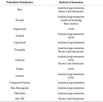
We have presented an up-to-date review of the activity time distributions used in PERT with highlights of various methods adopted for parameter estimation. From the review, three estimation approaches are outstanding, namely, Ana-lytical Approximation, Monte Carlo Simulation and SANs, see Table 1 for de-tails.
DOI: 10.4236/ajor.2017.76027 367 American Journal of Operations Research
Table 1. Summary of activity time distributions used in project network analysis.
Probability Distribution Method of Estimation
Beta Analytical approximation. Monte Carlo Simulation.
Normal Analytical approximation. Analytical bounding. Exact analysis.
Exponential SANs
Weibull Analytical approximation. SANs
Lognormal Analytical approximation
Triangular Analytical approximation. Monte Carlo Simulation.
Uniform Analytical approximation. SANs.
Monte Carlo Simulation.
Erlang SANs.
Gamma Analytical approximation. SANs.
Compound Poisson Analytical approximation
Beta-Rectangular Analytical approximation.
Tilted-Beta Analytical approximation.
Burr XII Monte Carlo Simulation
A basic advantage of the Simulation approach is that it allows the use of any activity time distribution. In short, different distributions can be used on differ-ent activities of the same project. It was observed that the choice of most of the activity time distributions was based on flexibility and convenience, with no clear empirical evidences, as earlier noted by Trietsch etal. [49]. This review also points to the fact that the beta distribution is not the sole activity time distribu-tion as presented in most basic texts and lecture notes on project managements.
The importance of appropriate choice of activity time distribution cannot be overemphasized, irrespective of the method adopted to estimate the parameters of project network. Hence, we suggest that practitioners, apart from using theo-retical information, should endeavor to make their choices of activity duration distributions based on particular empirical evidences and not just on simplicity. Developers of project management software should also incorporate many probability distributions as much as possible to enable users’ flexibility of choice. The information provided in this research can be used to extend the study by Hajdu and Bokor [8].
References
DOI:10.4236/ajor.2017.76027 368 American Journal of Operations Research
[2] Malcom, D., Roseboom, J. and Clark, C. (1959) Application of a Technique for Re-search and Development Program Evaluation. Operations Research, 7, 646-669.
https://doi.org/10.1287/opre.7.5.646
[3] MacCrimmon, K. and Ryavec, C.A. (1964) An Analytical Study of the PERT As-sumptions. Operations Research, 12, 16-37. https://doi.org/10.1287/opre.12.1.16 [4] Lootsma, F. (1989) Stochastic and Fuzzy PERT. European Journal of Operational
Research, 43, 174-183. https://doi.org/10.1016/0377-2217(89)90211-7
[5] Elmaghraby, S.E. (1977) Activity Networks: Project Planning and Control by Net-works. John Wiley & Sons, New York.
[6] Clark, C.E. (1962) The PERT Model for the Distribution of an Activity Time. Op-erations Research, 10, 405-406. https://doi.org/10.1287/opre.10.3.405
[7] Kamburowski, J. (1997) New Validations of PERT Times. International Journal of Medical Sciences, 25, 323-328. https://doi.org/10.1016/S0305-0483(97)00002-9 [8] Hajdu, M. and Orsolyo, B. (2014) The Effects of Different Activity Distributions on
Project Duration in PERT Networks. Procedia Social and Behavioural Sciences, 119, 766-775. https://doi.org/10.1016/j.sbspro.2014.03.086
[9] Williams, T.M. (1992) PERT Completion Times Revisited. INFORMS Transactions in Education,6, 21-34. https://doi.org/10.1287/ited.6.1.21
[10] Hahn, E.D. and Martín, M.M.L. (2015) Robust Project Management with the Tilted Beta Distribution. SORT, 39, 253-272.
[11] Abou Rizk, S. and Halpin, D. (1992) Statistical Properties of Construction Duration Data. Journal of Construction Engineering Management,118, 525-544.
https://doi.org/10.1061/(ASCE)0733-9364(1992)118:3(525)
[12] Mohan, S., Gopalakrishnan, M., Balasubramanian, H. and Chandrashekar, A. (2007) A Lognormal Approximation of Activity Duration in PERT Using Two Time Esti-mates. Journal of the Operational Research Society, 58, 827-831.
https://doi.org/10.1061/(ASCE)0733-9364(1992)118:3(525)
[13] Shankar, N.R., Babu, S.S., Thorani, Y.L.P. and Raghuram, D. (2011) Right Skewed Distribution of Activity Times in PERT. International Journal of Engineering Science and Technology, 3, 2932-2938.
[14] Van Slyke, R. (1963) Monte Carlo Methods and the PERT Problems. Operations Research,11, 839-860.https://doi.org/10.1287/opre.11.5.839
[15] PMBOK (2008) A Guide to the Project Management Body of Knowledge. 4th Edi-tion, Project Management Institute Inc., Newtown Square, Pennsylvania.
[16] Farnum, N. and Stanton, L. (1987) Some Results Concerning the Estimation of Beta Distribution Parameters in PERT. Journal of the Operational Research Society, 38, 287-290.https://doi.org/10.1057/jors.1987.45
[17] Grubbs, F.E. (1962) Attempts to Validate Certain PERT Statistics or Picking on PERT. Operations Research,10, 912-915.https://doi.org/10.1287/opre.10.6.912
[18] Premachandra, M. (2001) An Approximation of The Activity Duration Distribution in PERT. Computing and Operations Research, 28, 443-452.
https://doi.org/10.1016/S0305-0548(99)00129-X
[19] Herrerias-Velasco, J.M., Herrerias-Pleguezuelo, R. and Dorp, J.R.V. (2011) Revisit-ing the PERT Mean and Variance. European Journal of Operational Research,210, 448-451.https://doi.org/10.1016/j.ejor.2010.08.014
[20] Golenko-Ginzburg, D. (1988) On the Distribution of Activity Times in PERT.
DOI: 10.4236/ajor.2017.76027 369 American Journal of Operations Research https://doi.org/10.1057/jors.1988.132
[21] Nowpada, R.S. and Veeramachaneni, S. (2009) An Approximation for the Activity Duration Distribution, Supporting Original PERT. Applied Mathematical Sciences, 57, 2823-2834.
[22] Trout, M.D. (1989) On the Generality of the PERT Average Time Formula. Deci-sion Sciences,20, 491-412.https://doi.org/10.1111/j.1540-5915.1989.tb01888.x
[23] Arsham, H. (1993) Managing Project Duration Uncertainties. Omega,21, 111-122.
https://doi.org/10.1016/0305-0483(93)90043-K
[24] Donaldson, W.A. (1985) Estimation of Mean and Variance of a PERT Network.
Operations Research, 33, 862-881.
[25] Gallagher, C. (1987) A Note on PERT Assumptions. Management Science, 33, 1360.
https://doi.org/10.1287/mnsc.33.10.1360
[26] Healy, T.H. (1961) Activity Subdivision and PERT Probability Statements. Opera-tions Research, 9, 341-348.https://doi.org/10.1287/opre.9.3.341
[27] Littlefield, T.K. and Randolph, P.H. (1987) An Answer to Sasieni’s Question on PERT Times. Managements Science, 33, 1357-1359.
https://doi.org/10.1287/mnsc.33.10.1357
[28] Moder, J.J. and Rodgers, E.G. (1968) Judgment Estimates of the Moments of PERT Type Distributions. Management Science, 15, 76-83.
https://doi.org/10.1287/mnsc.15.2.B76
[29] Sasieni, M.V. (1986) A Note on PERT Times. Management Sciences, 32, 1652-1653.
https://doi.org/10.1287/mnsc.32.12.1652
[30] Perry, C. and Greig, I.D. (1975) Estimating the Mean and Variance of Subjective Distributions in PERT and Decision Analysis. Management Sciences,21, 1477-1480.
https://doi.org/10.1287/mnsc.21.12.1477
[31] Keefer, D.L. and Verdini, W.A. (1993) Better Estimation of PERT Activity Time.
Management Sciences,39, 1086-1091.https://doi.org/10.1287/mnsc.39.9.1086
[32] Kamburowski, J. (1985) Normally Distributed Activity Durations in PERT Net-works. Journal of the Operational Research Society,36, 1051-1057.
https://doi.org/10.1057/jors.1985.184
[33] Dodin, B. (1985) Bounding the Project Completion Time Distribution in PERT Networks. Operations Research,33, 862-881. https://doi.org/10.1287/opre.33.4.862
[34] Sculli, D. (1983) The Completion Time of PERT. Journal of Operational Research Society, 34, 155-158.https://doi.org/10.1057/jors.1983.27
[35] Drezner, Z. and Anklesaria, K.P. (1986) A Multivariate Approach to Estimating the Completion Time for PERT Networks. Journal of Operational Research Society,37, 811-815.https://doi.org/10.1057/jors.1986.140
[36] Cottrell, P.E. and Wayne, D. (1999) Simplified Program Evaluation and Review Technique (PERT). Journal of Construction Engineering and Management, 125, 16-22.https://doi.org/10.1061/(ASCE)0733-9364(1999)125:1(16)
[37] Kotiah, T.C.T. and Wallace, N.D. (1979) Another Look at PERT Assumptions.
Management Sciences, 20, 44-49.https://doi.org/10.1287/mnsc.20.1.44
[38] Maggot, J. and Skudlarski, K. (1993) Estimating the Mean Completion Time of PERT Network with Exponentially Distributed Duration of Activities. European Journal of Operational Research,71, 70-79.
https://doi.org/10.1016/0377-2217(93)90261-K
DOI:10.4236/ajor.2017.76027 370 American Journal of Operations Research
Duration for Stochastic Acyclic Networks. Journal of Indian Society of Statistics and Operations Research,19, 37-49.
[40] Abdelkader, Y.H. (2010) Adjustment of the Moments of the Project Completion Times when Activity Times are Exponentially Distributed. Annals of Operations Research,181, 503-514.https://doi.org/10.1007/s10479-010-0781-3
[41] Abdelkader, Y. (2006) Stochastic Activity Networks with Truncated Exponential Activity Times. Journal of Applied Mathematics and Computing, 20, 119-132.
https://doi.org/10.1007/BF02831927
[42] Cinicioglu, E.N. and Shenoy, P.P. (2009) Using Mixtures of Truncated Exponentials for Solving Stochastic PERT Networks. Proceedings of the Eighth Workshop on Uncertainty Processing (WUPES’09), Liblice, 19-23 September 2009, 269-283. [43] Azaron, A. and Modarres, M. (2007) Project Completion Time in Dynamic PERT
Networks with Generating Projects. Scientia Iranica, 14, 56-63.
[44] Kamburowski, J. (1985b) An Upper Bound on the Expected Completion Time of PERT Networks. European Journal of Operational Research,21,206-212.
https://doi.org/10.1016/0377-2217(85)90032-3
[45] Kulkarni, V.G. and Adlakha, V.G. (1986) Markov and Markov Regenerative PERT Networks. Operations Research,34, 769-781.https://doi.org/10.1287/opre.34.5.769
[46] Kwon, H.D., Lippman, A.S., McCCardle, K.F. and Tang, C.S. (2010) Project Man-agement Contracts with Delayed Payment. Mamufacturing and Service Operations Research, 12, 692-707.https://doi.org/10.1287/msom.1100.0301
[47] Abdelkader, Y.H. (2004) Evaluating Project Completion Times When Activity Times Are Webull Distributed. European Journal of Operational Research, 157, 704-715.https://doi.org/10.1016/S0377-2217(03)00269-8
[48] McCombs, E.L., Elam, M.E. and Pratt, D.B. (2009) Estimating Task Duration in PERT Using the Weibull Probability Distribution. Journal of Modern Applied Sta-tistical Methods, 8, 282-288. https://doi.org/10.22237/jmasm/1241137500
[49] Trietsch, D., Mazmanyan, L., Gevorgyan, L. and Baker, K.R. (2012) Modeling Ac-tivity Times by the Parkinson Distribution with a Lognormal Core: Theory and Va-lidation. European Journal of Operational Research, 216, 386-396.
https://doi.org/10.1016/j.ejor.2011.07.054
[50] Johnson, D. (1997) The Triangular Distribution as a Proxy for Beta Distribution in Risk Analysis. The Statistician, 46, 387-398.
https://doi.org/10.1111/1467-9884.00091
[51] Okagbue, H.I., Edeki, S.O., Opanugu, A.A., Oguntunde, P.E. and Adeosun, M.E. (2014) Using the Average of the Extreme Values of a Triangular Distribution for a Transformation, and Its Approximant via the Continuous Uniform Distribution.
British Journal of Mathematics and Computer Science, 4, 3497-3507.
https://doi.org/10.9734/BJMCS/2014/12299
[52] Abdelkader, Y.H. and Al-Ohali, M. (2013) Estimating the Completion Time of Sto-chastic Activity Networks with Uniform Distributed Activity Times. Archives Des Sciences, 66, 115-134.
[53] Kleindorfer, G.B. (1971) Bounding Distributions for a Stochastic Acyclic Network.
Operations Research,19, 1586-1601.https://doi.org/10.1287/opre.19.7.1586
[54] Bendell, A., Solomon, D. and Carter, J.M. (1995) Evaluating Project Completion Times When Activity Times Are Erlang Distributed. Journal of Operational Re-search Society,46, 867-882.https://doi.org/10.1057/jors.1995.118
DOI: 10.4236/ajor.2017.76027 371 American Journal of Operations Research
Networks. Kybernetica, 39, 347-358.
[56] Lootsma, F.A. (1966) Network Planning with Stochastic Activity Durations: An Evaluation of PERT. Statistica Neerlandica, 20, 43-69.
https://doi.org/10.1111/j.1467-9574.1966.tb00492.x
[57] Abdelkader, Y.H. (2004(b)) Computing the Moments of Order Statistics from Nonidentically Distributed Gamma Variables with Applications. International Journal of Mathematics, Game Theory and Algebra,14, 1-8.
[58] Parks, W. and Ramsing, K. (1969) The Use of Compound Poisson in PERT. Man-agement Science,15, 397-402.https://doi.org/10.1287/mnsc.15.8.B397
[59] Hahn, E. (2008) Mixture of Densities for Project Management Activity Times: A Robust Approach to PERT. European Journal of Operational Research, 18; 450-459.
https://doi.org/10.1016/j.ejor.2007.04.032
[60] Yachchali, S.H. (2011) A Simple Approach to Project Scheduling in Networks with Stochastic Durations. Proceedings of the World Congress on Engineering, 1, Lon-don, 6-8 July 2011.
[61] Topp, C.W. and Leone, F.C. (1955) A Family of J-Shaped Frequency Functions.
Journal of the American Statistical Association, 50, 209-219.
https://doi.org/10.1080/01621459.1955.10501259
[62] Burr, I.W. (1942) Cumulative Frequency Functions. Annals of Mathematical Statis-tics,13, 215-232.https://doi.org/10.1214/aoms/1177731607
[63] Udoumoh, E.F., Ebong, D.W. and Iwok, I.A. (2017) Simulation of Project Comple-tion Time with Burr XII Activity DistribuComple-tion. ARJOM, 6, 1-14.