Do Almost All Trees Have No Perfect Dominating Set?

ISSN Online: 2161-7643 ISSN Print: 2161-7635

DOI: 10.4236/ojdm.2018.81001 Nov. 27, 2017 1 Open Journal of Discrete Mathematics

Do Almost All Trees Have No Perfect

Dominating Set?

Bill Quan Yue

Sarasota, FL 34243, USA

Abstract

A graph G is said to have a perfect dominating set S if S is a set of vertices of G and for each vertex v of G, either v is in S and v is adjacent to no other vertex in S, or v is not in S but is adjacent to precisely one vertex of S. A graph G may have none, one or more than one perfect dominating sets. The problem of de-termining if a graph has a perfect dominating set is NP-complete. The prob-lem of calculating the probability of an arbitrary graph having a perfect do-minating set seems also difficult. In 1994 Yue [1] conjectured that almost all graphs do not have a perfect dominating set. In this paper, by introducing multiple interrelated generating functions and using combinatorial computa-tion techniques we calculated the number of perfect dominating sets among all trees (rooted and unrooted) of order n for each n up to 500. Then we cal-culated the average number of perfect dominating sets per tree (rooted and unrooted) of order n for each n up to 500. Our computational results show that this average number is approaching zero as n goes to infinity thus sug-gesting that Yue’s conjecture is true for trees (rooted and unrooted).

Keywords

Tree, Dominating, Graph, Generating Function

1. Introduction

A vertex v in a graph G is said to dominate itself and its neighbors. A set S of vertices in a graph G is said to be a dominating set for G if every vertex of G is dominated by at least one member of S. A set S of vertices in a graph G is said to be a perfect dominating set for G if every vertex of G is dominated by exactly one member of S. If a graph G with vertex set V has a perfect dominating set of

{

1, 2, , k

}

S= u u  u , then V can be partitioned into k subsets N u

( )

i ,

(

1≤ ≤i k

)

, where N u

( )

i is the set of vertex ui together with its neighbors, i.e.

How to cite this paper: Yue, B.Q. (2018) Do Almost All Trees Have No Perfect Do-minating Set? Open Journal of Discrete Mathematics, 8, 1-13.

https://doi.org/10.4236/ojdm.2018.81001

Received: March 7, 2017 Accepted: November 24, 2017 Published: November 27, 2017 Copyright © 2018 by author and Scientific Research Publishing Inc. This work is licensed under the Creative Commons Attribution International License (CC BY 4.0).

http://creativecommons.org/licenses/by/4.0/

DOI: 10.4236/ojdm.2018.81001 2 Open Journal of Discrete Mathematics

( )

1

i i

V N u

=

=



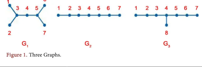
_{. The concept of perfect domination set in a graph has wide range} of applications. For example, resource allocation and placement in parallel computers [2], code error detecting and correcting [3]. In social networking context, if G is the graph presentation of a social network and if G has a perfect dominating set S, then the members of S are independent influencers that will completely influence the entire network, and each non-influencing member of G will be influenced by exactly one influencer from S. For such a social network G, if we can identify one perfect dominating set S, we can focus on S instead of entire social network when we want to influence, do campaign for instance, on the entire network. In the context of a common UNIX file system in which we consider only directories, a rooted tree T can be used to completely represent the entire file system. If we can configure T so that T has a perfect dominating set S, then each node in S can be assigned an agent, these agents are independent and can carry out monitoring or security checks on entire system in very efficient manner.

A graph can have none, one or more than one perfect dominating sets. See

Figure 1. In Figure 1, graph G1 has no perfect dominating set, G2 has one perfect dominating set {1, 4, 7} and G3 has two perfect dominating sets {1, 4, 7} and {2, 8, 6}.

For a graph G, three questions can be asked: “Does G have a perfect dominating set?” “If G has perfect dominating set(s), how many are there, what are they?” “What is the probability of one arbitrary graph G having a perfect dominating set?” The problem of determining if a graph has a perfect dominating set is NP-complete [4] [5], and the problem remains NP-complete even if the graphs are restricted to 3-regular planar graphs. Thus the problem of determining if a graph has a perfect dominating set is quite difficult. The second question also seems very difficult. For the third question, in 1994 Yue [1] conjectured that almost all graphs do not have a perfect domination set.

For a given tree, Livingston and Stout have obtained linear algorithms to answer the first question and the second question [6]. In this paper, we will focus on and study trees (rooted and unrooted) by using combinatorial computational techniques to answer a part of the second question (how many perfect dominating sets) and the third question from completely different standpoint.

From onwards unless otherwise stated, the trees considered are rooted and unrooted.

[image:2.595.203.536.627.738.2]

We first compute the number of perfect dominating sets among all trees of

DOI: 10.4236/ojdm.2018.81001 3 Open Journal of Discrete Mathematics order n for each n up to 500 then we calculate the average number of perfect dominating sets per tree of order less than or equal to n for each n up to 500. Since a tree can have at most finite number of perfect dominating sets, if this average number is approaching zero as n gets bigger then we can say that it provides computation evidence of Yue’s conjecture being true for trees.

Unlike other graph counting problems, it appears impossible to obtain recursive formulas for the number of perfect dominating sets among all trees directly. So, instead of using a single generating function, we introduce four interrelated generating functions and obtain recursive formula for each, then we use these formulas to find the number of perfect dominating sets among all trees of order n for each n up to 500. We then calculate the number of trees of order n for each n up to 500 and finally calculate the average number of perfect dominating sets per tree of order less than or equal to n for each n up to 500.

The notation and terminology in this paper follow that in Harary and Palmer

[7] and Chartrand [8]. In particular, Z S

( )

n =Z S s s

(

n; ,1 2,,sn

)

is the cycle index for the symmetric group Sn acting on n objects. This is a polynomial in n

variables s s1, 2,,sn. For any generating function g x

( )

, Z S g x

(

n;

( )

)

is a

shorthand representing the substitution

( )

( )

2

1 , 2 ,

s =g x s =g x  in Z S

( )

n . For related results see [2] and [3], for terminologies readers are referred to [7] [8] and [9].

2. Generating Functions for Rooted Trees

In order to compute the number of perfect dominating sets among all rooted trees we would like introduce four generating functions. We let

( )

1

n n n

P x P x

∞

=

=

∑

be the generating function in which Pn is the number of perfect dominating

sets among all rooted trees of order n. Unlike other graph counting problems, it is not possible to obtain recursive formulas for the number of perfect dominating sets among all trees directly, so we introduce other three interrelated generating functions.

Let

( )

1

n n n

R x R x

∞

=

=

∑

(1) be the generating function in which Rn is the number of perfect dominating

sets among all rooted trees of order n which have the root in the dominating set. (The root is dominated by itself.) We call these rooted trees as perfectly dominated rooted trees of type I.

Let

( )

1

n n n

C x C x

∞

=

=

∑

DOI: 10.4236/ojdm.2018.81001 4 Open Journal of Discrete Mathematics sets among all rooted trees of order n which have the root dominated by one of its children. (The root is dominated from inside.) We call these rooted trees as perfectly dominated rooted trees of type II.

We let the forth series be

( )

1

n n n

B x B x

∞

=

=

∑

(3) In this series B x

( )

, we would like to count sets that are nearly perfect

dominating sets among all rooted trees of order n. For each such a rooted tree T, we should like to count the sets with the property that for each such a set S, with the exception of the root, every vertex is perfectly dominated by a unique vertex in the set S. But the root is neither in S nor is it dominated by any vertex in S. Such a tree T is not perfectly dominated, but it can be a branch in a larger perfectly dominated tree of type I. (The root is dominated from outside.) We call these branches as branches of type B.

Observe that the number of perfect dominating sets among all rooted trees of order n equals the sum of perfectly dominated rooted trees of type I of order n and perfectly dominated rooted trees of type II of order n, i.e. Pn=Rn+Cn,

since for any perfect dominating set S, the root must either be in S or be dominated by one of its children.

Thus we have

( )

( )

( )

.

P x =R x +C x

(4) It may seem that B x

( )

is not involved in the process of counting the

number of perfect dominating sets, but we shall soon see we need it to calculate

( )

R x and C x

( )

.

3. Functional Relations among the Counting Series

Our object is to find the number of perfect dominating sets among all rooted trees of order n. In the previous section we saw that this number is equal to

n n

R +C . We first find the functional relations among R x C x

( ) ( )

, and B x

( )

then generate Rn and Cn for every n up to 500.

Theorem 1. For the functions introduced in (1), (2) and (3) the following equations hold:

( )

(

( )

)

0

, k k

R x x Z S B x

∞

=

 

= _

∑

_

(5)

( )

( ) ( )

C x =R x B x

(6)

( )

(

( )

)

0

, k k

B x x Z S C x

∞

=

 

= _

∑

_

DOI: 10.4236/ojdm.2018.81001 5 Open Journal of Discrete Mathematics tree of type II or branch of type B must have the property that it is built by a root and some (maybe none) branches of perfectly dominated tree of type I, or some (maybe none) perfectly dominated tree of type II or some (maybe none) branch type B.

Now we would like to examine the structure of rooted trees of perfectly dominated tree of type I, perfectly dominated tree of type II and branch of type B respectively.

For perfectly dominated tree of type I, any branch of perfectly dominated tree of type I is invalid since otherwise both root of the tree and root of the branch will be in the dominating set, contradicting the property of perfectly dominating set. Any branch of perfectly dominated tree of type II is invalid since otherwise the root of the branch will be dominated twice, contradicting the property of perfectly dominating set. On the other hand, it can have any number of branches of type B. See Figure 2.

This allows us to deduce the Equation (5):

( )

(

( )

)

0

, .

k k

R x x Z S B x

∞

=

 

= _

∑

_

In this expression, the factor x accounts for the root. Each Z S B x

(

k,

( )

)

allows for k branches of type B. Thus the structure shown in Figure 2 leads us to Equation (5).

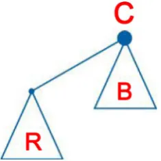
For rooted trees of perfectly dominated tree of type II, it must have exactly one branch of perfectly dominated tree of type I and the rest of it must be a branch of type B. See Figure 3.

[image:5.595.289.456.448.561.2]

That gives us the Equation (6):

Figure 2. The structure of rooted of perfectly dominated tree of type I.

[image:5.595.316.434.588.706.2]

[image:6.595.292.454.74.172.2]

DOI: 10.4236/ojdm.2018.81001 6 Open Journal of Discrete Mathematics

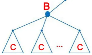
Figure 4. The structure of rooted tree of type B.

( )

( ) ( )

C x =R x B x

For a branch type B, any branch of perfectly dominated tree of type I is invalid since otherwise the root of the tree will be dominated, contradicting the property of branch of type B. It can have any number of branches of type type II. It cannot have any branch of type B since otherwise the root of the branch would not be dominated, contradicting the property of rooted tree of type B. See Figure 4.

So we have the Equation (7):

( )

(

( )

)

0

, .

k k

B x x Z S C x

∞

=

 

= _

∑

_

4. Recurrence Relations and Numerical Values

for Rooted Trees

Although the following two equations can be derived from (5) and (7) (see [7]), we would like to use combinatorial arguments to obtain them.

( )

(

2

)

1

1 k k Bk

k

R x x x x

∞

=

=

∏

+ + +_

(8)

( )

(

2

)

1

1 k k Ck

k

B x x x x

∞

=

=

∏

+ + +

(9) See Figure 2 again, we examine the following expression:

(

2

)

=1

1 k k Bk.

k

x x x

∞

+ + +

∏



In this expression, x counts the root. The number 1 represents no branch of order k; the term _xk represents one branch of order k, _x2k represents two

branches of order k, and so on. The number Bk represents the number of ways

to select a branch of type B of order k.

Then observe that the product of all these is, by the structure of perfectly dominated tree of type I, R x

( )

. That is Equation (8). By similar arguments, we

can get (9).

Knowing that R1=1, B1=1, C1=0, theoretically these recurrence relations allow us to compute Rn, Bn, Cn for any particular n. For example if we want

to calculate Rm, Bm, Cm, we only need to know Rn, Bn, Cn for each n up

DOI: 10.4236/ojdm.2018.81001 7 Open Journal of Discrete Mathematics By using (8), (9) and (6) on on a 64bit-based PC with a CPU process of T4200 (Pentium(R) Dual-Core) and RAM of 4 GB we can determine Rn, Bn, Cn for

each n up to 10 in 0.165 seconds, for each n up to 15 in 29.2 seconds and for each n up to 20 in 5719.8 seconds. At n equals 25, the same PC failed to manage the complexity of calculations. In order to determine Rn, Bn, Cn for each n

up to 500 more efficiently we need to modify (8), (9) and (6).

In Equation (8) we rewrite the geometric series and then use the binomial theorem with negative exponents to get

( )

(

)

(

)

2 1 1 0 1 1 1 1 . k k B k k k B k k k kl l k

R x x x x

x x B l x x l ∞ = ∞ ₋ = ∞ ∞ = = = + + + = − + −   = _{ }  

∏

∏

∑

∏



Similarly, from (9) we have

( )

0 1 1 . k kl l k C l

B x x x

l ∞ ∞ = = + −   = _{ }  

∑

∏

Formally expanding the product of two series in (6) gives

( )

1

2 1

. k

k l k l k l

C x R B x

∞ − − = =   = _{ }  

∑ ∑

To find out the formulas to calculate Rn, Bn, Cn for each n up to 500, we

first introduce some notation. Let

( )

0

n n n

f x f x

∞

=

=

∑

be any power series, then

( )

n

n

x f x f

  =

  . For example e

( )

1 ! n n x x n − −   =   .

Now suppose we would like to find R_m,B_m and C_m

(

2≤ ≤m 500

)

, then 1 1 0 1 1 m m k k m kl m l k B l

R x x x

l −     −   = =   + −       =_{    }      

∑

∏

1 1 0 1 1 m m k k m kl m l k C l

B x x x

l −     −   = =   + −       =_{    }      

∑

∏

1 1 . m

m k m k

k

C R B

− − =

=

∑

With the aid of the same computer and Mathematica, these three formulas provide Rn, Bn,and Cn for each n up to 500.

5. Equation and Numerical Values for Unrooted Trees

DOI: 10.4236/ojdm.2018.81001 8 Open Journal of Discrete Mathematics We have seen that (4):

( )

( )

( )

P x =R x +C x

is the generating function in which Pn is the number of perfect dominating sets

among all rooted trees of order n. We let

( )

1

n n n

p x p x

∞

=

=

∑

be the generating function in which pn is the number of perfect dominating

sets among all unrooted trees of order n.

Theorem 2. The counting series p x

( )

satisfies

( )

( )

1 2

( )

( )

2 . 2

p x =R x − _C x −C x _

(10)

Proof: We will use the following Theorem (Dissimilarity characteristic theorem for trees) due to Otter [10] and presented in [7].

For any tree T of order n

* *

1=n −q +s. ₍₁₁₎

In the equation *

n is the number of dissimilar vertices of T, or more precisely, the number of equivalence classes of vertices of T under action of the symmetric group of Sn;

*

q is the number of dissimilar edges of T, or more

precisely, the number of equivalence classes of edges of T under action of the symmetric group of Sn; s is the number of symmetric edges of T under action

of the symmetric group of Sn.

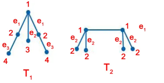
To illustrate the Theorem 2, we look the ordinary tree T1 and the ordinary tree T2 both of order 6 in Figure 5.

For tree T1, *

4

n = , q*=3 and s=0, so 1=n*−q*+s. For tree T₂,

*

2

n = , q*=2 and s=1, hence 1=n*−q*+s.

Observe that each unrooted tree T can give rise to exactly *

n different rooted trees and each unrooted tree T can be “rooted” at an edge in *

q

different ways. Also observe that for any unrooted tree T, two end vertices of a symmetric edge (if there is any) must be in the center of T. So s equals 0 or 1.

[image:8.595.251.522.575.712.2]

Now we apply Theorem 2 to our tree problem. Sum (11) over all unrooted

[image:9.595.260.500.60.126.2]

DOI: 10.4236/ojdm.2018.81001 9 Open Journal of Discrete Mathematics

Figure 6. Two valid ways of attaching two branches to an edge.

trees that have a perfect dominating set and that have exactly n vertices. The result is

* *

1= n − q + s

∑ ∑

∑

∑

but

∑

1=pn and *

n

n =P

∑

. Furthermore,

∑

_q* is the number of perfect dominating sets among all trees that are rooted at an edge and have the order of n. There are six possible ways to attach two branches to an rooted edge, i.e.

{

R R,

} {

, R B,

} {

, R C,

} {

, B B,

} {

, B C,

}

and

{

C C,

}

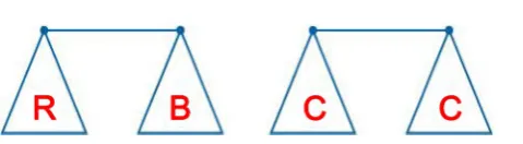
but only two ways are valid. First, if one branch is type R then another branch must be type B. Secondly, if one branch is type C then another branch must be type also C. See Figure 6.

Hence we have

( ) ( )

(

( )

)

*

2, .

q =R x B x +Z S C x

∑

Observe that for a tree that is rooted at an edge and s equals 1, then the two branches attached to the rooted edge must be exactly same two branches of type C, so

( )

2 _.

s=C x

∑

Finally, we have

( )

( )

( ) ( )

(

( )

)

( )

2

2, ,

p x =P x −_R x B x +Z S C x _+C x

or

( )

( )

( ) ( )

1 2

( )

( )

2

( )

2 . 2

p x =P x −R x B x − _C x +C x _+C x

Recalling that P x

( )

=R x

( )

+C x

( )

and C x

( )

=R x B x

( ) ( )

, we get (10):

( )

( )

1 2

( )

( )

2 . 2

p x =R x − _C x −C x _

We have Rn and Cn for every n up to 500 in hand, using (10) we can

determine pn for each n up to 500.

6. Enumeration Results

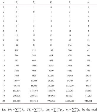
Enumeration results of R B C P_n, _n, _n, _n and p_n for each n up to 20 are presented in Table 1.

Using similar techniques we calculated the number rooted trees Tn of order

n for each n up to 500 and the number of unrooted trees tn of order n for each

[image:10.595.210.539.93.470.2]

DOI: 10.4236/ojdm.2018.81001 10 Open Journal of Discrete Mathematics

Table 1. Results of R B C Pn, n, n, n and pn (1≤ ≤n 20).

n Rn Bn Cn Pn pn

1 1 1 0 1 1

2 1 0 1 2 1

3 1 1 1 2 1

4 2 1 2 4 2

5 3 3 4 7 2

6 6 5 8 14 4

7 12 12 17 29 6 8 25 24 37 62 12 9 53 56 81 134 20 10 118 122 182 300 42 11 264 283 414 678 80 12 602 646 953 1555 169 13 1389 1516 2215 3604 347 14 3242 3546 5200 8442 755 15 7625 8421 12,291 19,916 1624 16 18,087 20,038 29,262 47,349 3611 17 43,161 48,085 70,069 113,230 8025 18 103,614 115,798 168,679 272,293 18,165 19 249,976 280,421 407,955 657,931 41,282 20 605,850 681,454 990,865 1,596,715 948,931

Let 1

k n

n k k

PP =

∑

=₌ P, TT_n=

∑

_kk n=₌₁T_k, pp_n=

∑

k n_k=₌₁p_k, tt_n=

∑

k n_k=₌₁t_k be the total number of perfect dominating sets among all rooted trees of order less than or equal to n, the total number rooted trees of order less than or equal to n, the total number of perfect dominating sets among all unrooted trees of order less than or equal to n and the total number unrooted trees of order less than or equal to n respectively, if PP TTn n is approaching zero as n getting larger then

we may assert that it is the computational evidence of Yue’s conjecture being true for rooted trees. For the same reason, if pp ttn n is approaching zero as n

getting larger then we may assert that it is the computational evidence of Yue’s conjecture being true for unrooted trees.

We can prove that (see [9] [11]) PP TTn n is approaching zero as n getting

larger whenever Pn is approaching zero as n getting larger and that pp ttn n

DOI: 10.4236/ojdm.2018.81001 11 Open Journal of Discrete Mathematics nth roots of n

n

P and n n

p since these two values can tell us the “rate” of Pn and pn approaching zero.

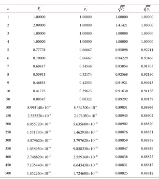
Results of Pn, pn, n Pn and n

n

[image:11.595.207.537.356.726.2]

p for each various n are presented in

Table 2.

7. Some Observations and Open Problems

From Table 2 we see n n

P and n n

p are approaching to about same value of 0.88 ... as n getting larger. Can we prove that they are actually convergent to the same limit? Can we find the limit?

We know for a perfect dominating set of rooted tree, the root is either dominated by itself or by one of its children, hence the number of perfect dominating sets among all rooted trees of order n is Pn=Rn+Cn (4). We may

ask what is the contribution of Rn (or Cn ) to Pn? The ratio of R Pn n

measures the contribution of Rn to Pn.

We have seen the average number of perfect dominating sets per rooted tree

n

P is somewhat bigger than the average number of perfect dominating sets per

unrooted tree pn. Another interesting question to ask is on what percentage

Table 2. Results of Pn, pn, nPn and n

n

p for each various n.

n Pn pn nPn

n n p

1 1.00000 1.00000 1.00000 1.00000 2 2.00000 1.00000 1.41421 1.00000 3 1.00000 1.00000 1.00000 1.00000 4 1.00000 1.00000 1.00000 1.00000 5 0.77778 0.66667 0.95098 0.92211 6 0.70000 0.66667 0.94229 0.93466 7 0.60417 0.54546 0.93054 0.91705 8 0.53913 0.52174 0.92568 0.92190 9 0.46853 0.42553 0.91921 0.90943 10 0.41725 0.39623 0.91630 0.91158 50 0.00347 0.00322 0.89292 0.89159 100 _{8.995140 10×} −6 _{8.364300 10×} −6 _{0.89031 0.88966}

150 8

2.333520 10× − 8

2.171050 10× − 0.88945 0.88902

200 _{6.055720 10×} −11 _{5.635600 10×} −11 _{0.88902 0.88870}

250 13

1.571730 10× − 13

1.462930 10× − 0.88876 0.88851

300 _{4.079620 10×} −16 _{3.797620 10×} −16 _{0.88859 0.88838}

350 18

1.058950 10× − 18

9.858330 10× − 0.88847 0.88829

400 _{2.748820 10×} −21 _{2.559160 10×} −21 _{0.88838 0.88822}

450 24

7.135440 10× − 24

6.643430 10× − 0.88831 0.88817

[image:12.595.213.538.95.456.2]

DOI: 10.4236/ojdm.2018.81001 12 Open Journal of Discrete Mathematics

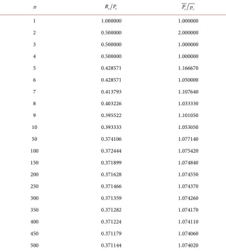
Table 3. Results of Rn Pn , Pn pn for each various n.

n R Pn n P pn n

1 1.000000 1.000000 2 0.500000 2.000000 3 0.500000 1.000000 4 0.500000 1.000000 5 0.428571 1.166670 6 0.428571 1.050000 7 0.413793 1.107640 8 0.403226 1.033330 9 0.395522 1.101050 10 0.393333 1.053050 50 0.374106 1.077140 100 0.372444 1.075420 150 0.371899 1.074840 200 0.371628 1.074550 250 0.371466 1.074370 300 0.371359 1.074260 350 0.371282 1.074170 400 0.371224 1.074110 450 0.371179 1.074060 500 0.371144 1.074020

does one rooted tree can give rise to more perfect dominating sets than that of one unrooted tree? The ratio of Pn pn measures the difference.

Results of R Pn n, Pn pn for each various n are presented in Table 3. From

Table 3 we see about 37% of perfect dominating sets for rooted trees in which the root is dominated by itself. On average per tree, rooted trees can give rise to about 7% more perfect dominating sets than unrooted trees.

DOI: 10.4236/ojdm.2018.81001 13 Open Journal of Discrete Mathematics

References

[1] Yue, B. (1994) Almost all Graphs Do Not Have a Perfect Domination Set, Personal Notes.

[2] Livingston, M.L. and Stout, Q.F. (1988) Distributing Resources in Hypercube Computers. Proceedings of the 3rd Conference on Hypercube Concurrent Com-puters and Application, Pasadena,19-20 January 1988, 222-231.

https://doi.org/10.1145/62297.62324

[3] Hamming, R.W. (1950) Error Detecting and Error Correcting Codes. The Bell Sys-tem Technical Journal, 29, 147-160.

https://doi.org/10.1002/j.1538-7305.1950.tb00463.x

[4] Garey, M.R. and Johnson, D.S. (1979) Computers and Intractability: A Guide to the Theory of NP-Completeness. W. H. Freeman & Co., New York.

[5] Johnson, D.S. (1985) The NP-Completeness Column: An Ongoing Guide. Journal of Algorithms, 6, 434-451.https://doi.org/10.1016/0196-6774(85)90012-4

[6] Livningston, M. and Stout, Q.F. (1990) Perfect Dominating Sets. Congressus Nu-merantium, 79, 187-203.

[7] Harary, F. and Palmer, E.M. (1973) Graphical Computation. Academic Press, New York.

[8] Chartrand, G. and Lesniak, L. (1986) Graphs and Digraphs. 2nd Edition, Wads-worth and Brooks/Cole, Monterey, CA.

[9] Rudin, W. (1976) Principles of Mathematical Analysis. McGraw-Hill, Boston. [10] Otter, R. (1948) The Number of Trees. Annals of Mathematics,49, 583-599.

https://doi.org/10.2307/1969046