Munich Personal RePEc Archive
Innovation and Income Inequality: World
Evidence
Benos, Nikos and Tsiachtsiras, Georgios
University of Ioannina, Universitat de Barcelona
7 February 2019
Online at
https://mpra.ub.uni-muenchen.de/92050/
1
Innovation and Income Inequality: World Evidence
Nikos Benos
*†Georgios Tsiachtsiras
Abstract
In this paper we explore the effect of innovation on income inequality using annual country panel data for 29 countries. We demonstrate that innovation activities reduce personal income inequality by matching patents from the European Patent Office with their inventors. Our findings are supported by instrumental variable estimations to tackle endogeneity. The results are also robust with respect to various inequality measures, alternative quality indexes of innovation, truncation bias, the use of patent applications together with granted patents and different ways to split or allocate patents.
JEL classification: D63, O30, O31, O33, O34, O40, O47
Keywords: top income inequality, overall inequality, innovation, citations, knowledge spillovers
Contact Information: Benos: Assistant Professor, Department of Economics, University of Ioannina, Ioannina 45110, Greece. Phone (+30)2651005955, Fax (+30)2651005092, E-mail: nbenos@cc.uoi.gr (corresponding author). Tsiachtsiras:
PhD student, School of Economics, Universitat de Barcelona, Barcelona 08034, Spain. Personal phone (+30)6980956826,
E-mail: ec002543@gmail.com. ORCID ID: 0000-0001-5026-6972.
Acknowledgements: We would like to thank Ernest Miguelez and Rosina Moreno Serrano for their suggestions. Also we
would like to thank Anastasia Litina for very helpful comments and discussions. In addition we would like to thank
Evangelos Dioikitopoulos, Dimitrios Dadakas and Nikos Tsakiris as well as the participants of the 4th International
Conference on Applied Theory, Macro and Empirical Finance (University of Macedonia, 2018) for their comments and
suggestions. We would also like to show our gratitude to the Science, Technology and Innovation Microdatalab of OECD
2
1
Introduction
Since the famous work of Solow (1956) economists have been studying the issues of growth and convergence. Many years later, Mankiw et al. (1992) use cross country data to test the Solow model. Their empirical analysis confirms the implications of Solow and claims that human capital is one of the most important growth determinants. Currently, country and regional income disparities are still high on the research agenda. It has been shown that economies at similar income levels often share many common elements like: education levels, science and technology endowments, infrastructure and institutional quality (Iammarino et al., 2018). Martin (2002) finds that even though within-country inequality has increased, there is a decline in across country-income inequality. He concludes that “the best strategy to reduce world income inequalities is to induce aggregate economic growth in poor
countries”. There is also a rich literature which argues that innovation is a major
determinant of economic growth (Aghion and Howitt, 1992 and Aghion and Jaravel, 2015). In this paper, we conclude that innovation activities reduce personal income
inequality in a world panel of countries (see also Antonelli and Gehringer, 2017).
3
[Insert Figure 1 here]
In Figure 2 we present a scatter plot of the log differences of citation years and top 1% income share. The countries1 with the red label have experienced an increase in citations per capita and at the same time a drop in their top 1% income share. Five of these eight countries, belong to the top fifteen most innovative countries based on Table 2. This evidence and the work of Aghion et al. (2018) about top income inequality in USA have inspired us to test the effect of innovation on top income inequality at the country level using a world sample.
[Insert Figure 2 here]
In this paper, we conclude that innovation is negatively associated with personal income inequality. We apply the same methodology with Aghion et al. (2018) with two differences: i) our sample contains countries instead of US states ii) we use patents from EPO, while they use patents from USPTO. Initially, we use OLS regressions with country and year fixed effects to explore this relationship across different countries over time. We also apply instrumental variable estimations to check the robustness of our basic results and confirm that causality runs from innovation to income inequality. Our main contributions in the literature are three. First, we contribute to the literature on inequality and growth by studying innovation as a channel linking the two (Aghion and Howitt, 1992 and Benos and Karagiannis, 2018). Second, we enrich the research on innovation and income inequality by
including many different measures of both innovation and income inequality (Aghion
1
4
at el., 2018). Third, we identify an innovation network through citations based on the
location of the inventors for the period 1978-1985. This knowledge based instrument helps us to tackle the endogeneity problem. Four papers are close to our work: the paper of Antonelli C. and Gehringer A. (2017), Risso and Carrera (2018), Wlodarczyk (2017) and Permana et al., (2018). Only Antonelli C. and Gehringer A. (2017) state that innovation may reduce income inequality2. We distinguish our paper from them by using quality measures of innovation3 and in addition two different instruments to deal with endogeneity. To the best of our knowledge, we are the first to present robust evidence according to which there is a causal effect of innovation on income inequality at the country level.
The rest of the paper is organized as follows. Section 2 explores the relations between innovation and income distribution. Section 3 presents the data. Section 4 shows the empirical strategy. Section 5 discusses the results and Section 6 concludes.
2
Theoretical framework
2.1 Innovation and Regional Inequality
According to many studies innovation has a positive effect on income inequality using regional data. First, there is the productivity effect which boosts wages of employees who work in innovative firms (Lee, 2011). These firms are able to develop new products and as a result new jobs are created (Breau et al., 2014). The
2
As we explain in the section 2, the other studies find positive results (Permana et al., 2018) or contradictory results for different measures of innovation (Wlodarczyk, 2017) or contradictory results for different amounts of the same measure of innovation (Risso and Carrera, 2018).
3
5
new jobs require advanced technologies suitable only for high skilled employees and this impact shows up in their salaries (Lee, 2011 and Breau et al., 2014). Also, innovative regions lure highly skilled and highly paid workers (Lee, 2011). Paas (2012) use GDP per capita in 2007 at the NUTS 2 level as explanatory variable and human capital indicators4, patent applications and R&D expenditures as independent variables. The cross region analysis shows that innovation has significant role in explaining regional income disparities between the EU NUTS2 regions.
The effect of innovation is stronger on top income shares than the rest of the income distribution (Aghion et al., 2018). According to them, innovation from both incumbents and entrants increases top income inequality. The difference between incumbents and entrants is that incumbents erect barriers. The barriers discourage new entrants and boost top income inequality. Pollak (2014) shows that incumbent firms defend their leading position by innovating at a high rate. His endogenous growth model justifies a persistent high growth rate by raising R&D intensity. This procedure stops only when the profits of the incumbent company fall.
Aghion et al. (2018) propose an additional channel through which innovation affects top income inequality. This channel is capital gains. The source of capital gains is the award for the innovative companies (mark-up). They indicate that through mark-up the companies have managed to increase their profits during the past forty years. Entrepreneurs and CEOs earn the bigger share of profits.
4
6
There are empirical findings, which confirm all above arguments. Lee (2011) uses data from the European Community Household Panel for the period 1995-2001 and finds that innovation has a positive effect on income inequality. Aghion et al. (2018) conclude that innovation drives top income inequality and not the opposite in US states by applying IV regressions. The results are similar for Canadian cities (Breau et al., 2014). In addition, innovation increases the inter-city inequality. Berkes and Gaetani (2018) explore the effect of innovation on income segregation within commuting zones5. Their main hypothesis is whether CZs that experience an expansion in innovation and knowledge activities also experience an increase in income segregation, defined as variation of income across neighborhoods within the city. Their results suggest that more innovative cities are also cities with higher levels of earnings inequality.
Liu and Lawell (2015) support that there is a U-shaped relationship between innovation and income inequality in Chinese provinces. They state that small amounts of innovation can reduce income inequality but big amounts actually increase it following the same methodology with Lee and Pose (2013). Another paper on the effect of innovation on income inequality in China is by Fan et al. (2012) who find that innovation and inequality increased at both regional and provincial levels. In a recent study, De Paolo et al., (2018) show that innovation increases top income shares but reduces overall income inequality.
The above studies provide theoretical channels through which innovation may reduce income inequality. Innovation creates knowledge spillovers (Aghion et al.,
5
7
2018), which can benefit individuals with fewer skills (Lee and Pose, 2013). These
individuals can learn from their high skilled partners and augment their productivity (Lee, 2011). They then manage to increase their salaries and income inequality falls. However the empirical studies conducted at the regional level do not confirm the above arguments. One possible explanation is that geographical proximity may not be so important factor as other forms of proximity are (Boschma, 2005). Based on this framework we construct our spillover instrument in a next section.
2.2 Innovation and Cross-Country Inequality
8
Risso and Carrera (2018) find that the level of R&D should be high enough to reduce income inequality using the Gini index from the Standardized World Income Inequality Database and R&D as a percentage of GDP from the World Development Indicators as their measure of innovation. In any other case R&D will increase income inequality. Wlodarczyk (2017) employs also R&D expenditures and finds that R&D increases income inequalities, while EPO patent applications reduce income inequalities. Permana et al., (2018) adopt also EPO patent applications as a measure of innovation and find that innovation increases income inequality. The last two papers use European country samples with similar time periods6 and produce very different results.
Innovation may have different results in countries with dissimilar institutions. For example, Scandinavian countries prefer egalitarian societies (Acemoglu et al., 2012). Also, in contrast with many European countries, the flexible US markets allow
high skilled individuals to enter innovative sectors (Lee and Pose, 2013).
Chu A. and Cozzi G. (2017) create a theoretical model about patent policy and R&D subsidies. They examine the effects of these policies on income inequality in a Schumpeterian growth framework and find that these two policies produce very contradictory results. They conclude that strengthening patent protection causes a moderate increase in income inequality whereas raising R&D subsidies causes a large decrease in income inequality. In addition Jones and Kim (2018) develop a different Schumpeterian model. They claim that there are forces which boost top income shares by increasing the productivity of entrepreneurs but other forces enhance the creative
6
9
destruction effect. They argue that globalization may increase entrepreneurs’ profits but at the same time it increases competition.
2.3 Inequality and Innovation
Also inequality can affect innovation. A decrease in inequality may trigger an increase in the number of customers who can buy new products (Hatipoglu, 2012).
The change in inequality can affect the inventors’ expected profits and their decisions
about R&D investments.
On the contrary, Tselios (2011) finds that income inequality affects positively innovation at the NUTS 1 level. He states that there two opposite effects: i) the market size effect, i.e. an unequal distribution of income is responsible for small regional markets for new products and those markets grow slowly, as only a small number of consumers can afford to buy them; ii) the price effect, which implies that inequality can boost innovation because the richest consumers are willing to buy new products (Pose and Tselios, 2010).
These papers underlie the potential endogeneity problem between innovation and income inequality, which we try to solve in a next section. In general innovation has an ambiguous effect on income inequality, which depends on the level of aggregation of the analysis. It seems that innovation increases inequality using regional data, but reduces it when employing country-level data.
10
The data on pre-tax income shares of the top 10%, 1% and 0.5% income
earners in our country panel analysis are drawn from the World Wealth and Income Database (Alvaredo et al., 2017). These data are available for some countries from 1870 to 2016 but we focus on the period after 1978. We have chosen the Standardized World Income Inequality Database (Frederick Solt, 2016) for the Gini index like Risso and Carrera (2018). The Standardized World Income Inequality Database provides us with 100 equivalent Gini indexes for the pre-tax income and every of these has a different standard deviation. We include in our analysis the Gini index with the smallest standard deviation.
Quantity and quality measures of innovation come from The Science, Technology and Innovation Microdatalab of OECD. It has provided us with the databases containing quality and quantity measures of innovation on EPO7 patents. We use the OECD Patent Quality Indicators database, which includes the following quality measures of innovation: citations, claims, generality index and the family size of each patent and the OECD REGPAT database, which provides the location of inventors and applicants. Our quantity measures of innovation are the number of patents in the OECD Patent Quality Indicators database. When a patent has more than one inventor we split the patent equally among inventors (Aghion et al. 2018). We also use the applicants8 instead of inventors as a robustness check in the Appendix. We match the quality measures of innovation with the inventors without splitting them.
7
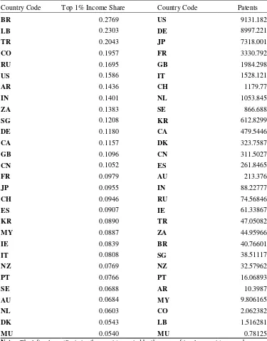
We use EPO databases because out of 29 countries in our sample 12 are European countries. Still, as we can see in Table 2, US have the biggest share of patents in the database and Japan is third.
8
11
We consider patents granted for our benchmark analysis. This is our first check for the quality of patents because good applications are more likely to be approved than bad ones (Régibeau and Rockett, 2010). In the Appendix we show that our results are robust even if we use the full sample (grants plus applications). In any case the number of patents is a crude measure of innovation because a patent with a great contribution to the literature and a patent with small contribution receive the same weight (Aghion et al., 2018).
For this reason, we apply quality measures of innovation, except the number of patents. The measures for our benchmark analysis are:
Patents per capita weighted by the number of citations within 9 years: this
variable measures the number of citations received within years after the application date (Aghion et al., 2018).
Patents per capita weighted by the number of claims: the number of claims
captures the breadth of a patent (Lerner, 1994 and Akcigit et al., 2016).
Patents per capita weighted by their generality index. The generality index is
based on a modification of the Hirschman-Herfindahl Index and uses information about the number and distribution of citations received and the Technology classes (IPC)10 of the patents these citations come from (Squicciarini et al., 2013).
9
The can be 5 or 7 years. We use 5 years window in our main analysis but we apply also the 7 years window in the Appendix.
10
They consider all IPC classes contained in the citing patent documents and account for the number and distribution of both 4-digit and n-digit IPC technology classes contained in citing patents, where n
12
Patents per capita weighted by family size. The family size is represented by
the number of patent offices at which a given invention has been protected. The most valuable patents are being protected by many different patent offices (Squicciarini et al., 2013).
The time span for all our innovation measures is 1978-2015. We use the filing date of the application. We use the patents which have been granted and different quality measures of innovation. We aggregate them at the country level and then divide them by the population of each country.
Many studies focus on citation indexes. The work of Hall et al. (2001) with citation data provided economists with the necessary tools to study the technological knowledge flows between inventors, companies and regions by using the citing and the cited patent. However there are some major problems in the citation data. First, there is truncation bias due to the time lag between application and grant (Aghion et al. 2018). Even though our measures of citations do not suffer much from truncation
bias11 we provide Table A10 in the Appendix where we restrict our sample until 2007 and our results are robust. Recent studies point a second problem in citation data, which is due to the similarity between patents. For instance Kelly et al., (2018) use the example of the famous patent of Nikola Tesla in 1888 with number 381,968 about AC motor. Despite the novelty of the patent it has received only two citations. The authors develop an alternative measure of innovation which captures the novel words in the description of the patents. In our paper we use alternative measures of innovation which are not based on citation data as claims and family size for our benchmark
11
13
analysis and include four additional measures in the Appendix. Still citation measures are the most famous and through them we track down the spillovers for subsequent innovations (Abrams et al., 2013).
We extract the rest of the control variables from the World Bank database. We have used the domestic credit (provided by financial sector as a percentage of GDP) to control for the financial sector influence on inequality. The financial sector usually helps the inventors to innovate and increase their salaries (Aghion et al., 2018). For instance, a big share of the employees (almost 27%) who belong in the top 0.1% income share in the United States work in the financial sector or use financial services (Szymborska, 2016). The second variable is general government final consumption expenditure (% of GDP) in order to control for the effect of government size in each country. Empirical studies find that government size has a negative effect on capital income inequality and specifically on the top 1% income share (Luo et al., 2017). Next we include in our analysis GDP per capita (constant 2010 US$), because
it has been found that GDP per capita has a positive effect on Gini index and the highest quintile income shares (Barro, 2008). We also control for the business cycle by using the unemployment rate (Aghion et al., 2018) and include population growth. We end up with an unbalanced panel of 29 countries over the time period 1978-2015.
4
Empirical Strategy
14
Our estimation method is similar with that of Aghion et al., (2018). We take the log of our innovation measures, inequality and GDP per capita and estimate the following equation:
where stands for country i, stands for time period t, is the measure of inequality
(in log), is the constant, , correspond to country and year fixed effects, is innovation in year (also in log) and, are the control
variables. We use country and year fixed effects to account for permanent cross-country differences in inequality and overall changes in inequality respectively. The advantage by taking both measures of inequality and innovation in logs is that can be interpreted as the elasticity of inequality with respect to innovation. We estimate autocorrelation and heteroskedasticity robust standard errors in all regressions.
We have decided to take the one year lag of innovation as the main independent variable. Our database, Patent Quality Indicators, provides us with the application dates of the patents. We include in our analysis patents from the European Patent Office. Depalo and Addario (2014) use the EPO patents Database and find that
inventors’ earnings peak at instead of . They assume that bureaucracy is
15
4.2 Endogeneity and Spillover Instrument
As it has been pointed in subsection 2.3 inequality can also boost innovation. Here, we argue that there is a casual effect from innovation on income inequality. Our first instrument accounts for the spillover effects of innovation. We claim that past innovation predicts and facilitates recent innovation. Knowledge creation boosts inequality, while knowledge diffusion through linkages and networks creates new opportunities (Iammarino et al., 2018). We build our citation network based on the location of the inventors. We want to capture the existence of spillovers among inventors (Aghion and Jaravel, 2015).
We follow the methodology of Aghion et al., (2018) to construct our spillover instrument. We use the OECD Citations database. The intuition is to instrument innovation in a country by its predicted value, based on past innovation intensities in other countries and the propensity to cite patents from these other countries (Aghion et al., 2018), (Technical details on the construction of the instrument are provided in
the Appendix). A second study of Berkes and Gaetani (2018) use a similar approach with the paper of Aghion et al., (2018). They split their sample of patents in 1994 and they use the old sample (from 1985-1994) to predict innovation activity in more recent years (2005-2014).
16
countries, so we do not worry much about this problem. However someone may claim the exactly opposite that long distances among countries makes difficult the diffusion of knowledge. According to many studies geographical proximity is not the reason for knowledge spillovers or innovation diffusion. The necessary conditions for knowledge to travel are the existence of strong organizational channels (such as firms) and, dense knowledge community networks and skills and this is exactly what we aim to capture by our spillover instrument (Breschi and Lissoni, 2001; Boschma, 2005; D’Este et al., 2013).
The second point is the predicting power of the instrument for recent innovation activity. Cohen and Levinthal (1989) introduce the notion of absorptive capacity and claim that knowledge spillovers can induce complementarities in R&D efforts (Aghion and Jaravel, 2015). According to Aghion and Jaravel (2015) innovation in one country is often built on knowledge created by innovations in another country. Malerba et al., (2013) use patent data from EPO and find that international R&D spillovers are effective in fostering patenting. Citations reveal past knowledge spillovers and provide channels for future innovation (Caballero and Jaffe, 1993). Also, spillovers reduce the cost of innovation (Aghion et al., 2018). Our first
stage results from Table A5 in the Appendix confirm the strength of our instrument. The coefficient of our spillover instrument is positive and significant when we use either quantity or quality measures of innovation.
17
checks in Table A7 of the Appendix. Our instrument is based on the links between citing and cited patents until 1985. We exclude from the sample first all years before 1985 and then all years before 1987 to eliminate any doubts. Our measures of innovation remain significant. We take the one year lag of our instrument like (Aghion et al., 2018) to avoid any concerns about demand shocks.
4.3 Robustness Checks
In this section, we apply a second instrument as a robustness check. Our
second instrument is the log of “charges for the use of intellectual property, receipts
(BoP, current US$)” from International Monetary Fund. Our argument is that
countries which possess patents of high quality are going to receive bigger amounts of money for the authorized use of proprietary rights such as patents, trademarks, copyrights, industrial processes and designs including trade secrets and franchises. This is the first reason why we are interested on the receipts and not payments. Intellectual property rights have a positive effect on measures of innovation. Strong protection stimulates innovative activity and increases innovation incentives (Kanwar and Evenson, 2003 and Beladi et al., 2016). Kanwar and Evenson (2003) find that intellectual property protection has a positive effect on R&D expenditures, while Beladi et al., (2016) claim that strategic IPRs enforcement can be used as an effective
18
limited evidence that IPR boosts domestic innovation. Also Chu and Cozzi (2017) state that patent protection and R&D subsidies are two important policy instruments that determine technological progress and economic growth. Aghion et al., (2015) find that the product market reform, which took place in EU in 1992, facilitated
innovative investments in manufacturing industries of countries with strong patent
rights. They found a complementarity between competition and patent protection by
using a theoretical and an empirical model. This policy helped the industries with
strong patent rights to increase their R&D investments. The literature confirms the positive relationship between IPR and innovation.
Next we examine if this instrument is exogenous to income inequality. Here is
the second reason why we use receipts. The “charges for the use of intellectual
property, receipts” come from non-residents. At the country level this means that this
amount of money enters the domestic market from a foreign country. So, we believe that this instrument correlates directly only with our measures of innovation and it is unlikely to affect other domestic variables. To avoid any suspicions that our variable could potential affect indirectly our measures of inequality we use the lead of the variable as instrument. By using the periods for our instrument we believe that the case for it being exogenous with regard to income inequality in period is even
stronger. There is a second reason for using the value of our instrument. The average time for a patent to be granted in the EPO was almost 4 years in the 2005 (45.3 months, source: EPO official website). So, we apply the year to the application date in our model and use years of our instrument.
19
5.1 Summary Statistics and OLS Results
In this section we present the results from both OLS and IV regressions. All variables are defined in Table 1. We provide the sample of countries in Table 2 sorted both by the number of patents and top income share. Then, we present summary statistics in Table 3. In Table 4 we provide descriptive statistics for the measures of innovation and inequality for two distinctive years. It is clear that there is a significant increase in the means of our measures of inequality from 1985 to 2005. Also the minimum and maximum values have increased over these years. We reach the same conclusion also from the table with the innovation measures.
[Insert Table 1 here]
[Insert Table 2 here]
[Insert Table 3 here]
[Insert Table 4 here]
20
window keep the negative effect but at the 5% level of significance. We also provide in Tables A3-A4 of the Appendix alternative measures of innovation as robustness checks with robust and clustered standard errors respectively.
[Insert Table 5 here]
In Table 6, we test the effect of innovation on different measures of inequality. It is clear from this Table that innovation influences top income shares. We provide the most widely used measures of overall inequality and Gini index. Innovation has a negative coefficient, so innovation reduces not only top income but also overall income inequality.
[Insert Table 6 here]
5.2 IV Results
In Table 7 we present evidence after we use the spillover instrument. We see that now all measures of innovation are significant and have a negative effect on the top 1% income share. For instance a 1% increase in the citations within a 5 year window is associated with a 0.0402% fall of the top income share. In Table A8 of the Appendix we apply alternative measures of innovation with the spillover instrument
and the effect is again negative and significant.
21
Next, in Table 8 we present our results when we use as instrument the charges of intellectual property rights. A 1% increase in the citations within a 5 year window reduces the top 1% income share by 0.0813%. Again in Table A9 we provide different measures of innovation with our second instrument and the results confirm the negative and significant effect of innovation.
[Insert Table 8 here]
In Table 9 we use both our instruments. Again we show that innovation measures have a negative impact on top income inequality. Our test statistics confirm that our instruments are appropriate.
Table 10 regresses the various measures of inequality on our measure of innovation (citation on a 5-year window). Innovation influences negatively the top 10% and top 0.5% income shares. Also, we see in column 5 that citations have a negative and significant effect on the Gini index. In Table A11 of the Appendix we use claims as measures of innovation and the spillover instrument. We get similar results as in Table 10.
[Insert Table 10 here]
5.3 Additional Findings and Discussion
22
5. Aghion et al. (2018) state that a good reason could be the interaction between innovation and competition. This explanation is based on the inverted-U relationship between these two variables (Aghion et al., 2005).
The government size and unemployment rate are also significant and with the expected signs. Both variables are in percentages (between 0-1) and indicate that a 1% increase in the government size, decreases the top 1% income share by 2.383% (Table 7), while the same increase in unemployment rate increases the top 1% income share
by 0.959% (column 2). In contrast with Aghion et al. (2018) we find strong evidence that government size and unemployment rate have the strongest effects, while the financial sector has a weaker effect. This is not surprising if we consider that in our sample 12 out of 29 countries are European. Even though Nickell (1997) states that there are big differences among European countries, we cannot ignore the fact that unemployment rate is very high in Europe (Fanti and Gori, 2011) and many European countries (high GDP countries) have higher than the optimal level of government size compatible with GDP growth rate maximization (Forte and Magazzino, 2011).
In the Second Appendix we present additional IV results when we use the full sample of patents12 and also when we match patents with applicants. More details about the construction of these databases can be found in the Appendix. We apply both our instruments in these regressions. We use the full sample in Table S2 and the applicants in Table S4 of the Second Appendix. Again the effect of innovation on income inequality is negative and significant.
12
23
6
Conclusions
To the best of our knowledge, we make the first attempt to explore the effect of innovation on top income shares at the country level and provide robust evidence accounting for endogeneity. In addition, our results are robust with respect to alternative inequality measures, quality indexes of innovation, truncation bias, the use of patent applications together with the granted patents and different ways to split or allocate the patents.
We identify a network of inventors through citations and our spillover instrument predicts recent innovation activity. We show that knowledge can be transferred between countries. The mobility of the inventors is a very crucial topic because they contribute to the diffusion of knowledge between different places (Miguelez., 2013 and Miguelez., 2018) .
24
data on income shares13 at the country level. Finally, an extension of the analysis could include property rights Tebaldi and Elmslie (2013) or taxation Akcigit et al. (2016) as additional control variables.
13
25
FIGURE 1
26
FIGURE 2
27
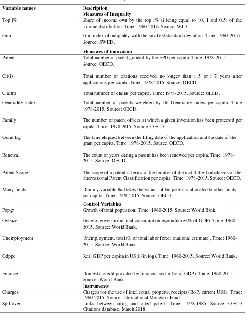
[image:28.595.61.569.38.691.2]TABLE 1
Variable description and notation
Variable names Description
Measures of Inequality
Top i% Share of income own by the top i% (i being equal to 10, 1 and 0.5) of the income distribution. Time: 1960-2016. Source: WID.
Gini Gini index of inequality with the smallest standard deviation. Time: 1960-2016. Source: SWIID.
Measures of innovation
Patent Total number of patent granted by the EPO per capita. Time: 1978-2015. Source: OECD.
Cit(i) Total number of citations received no longer than i=5 or i=7 years after applications per capita. Time: 1978-2015. Source: OECD.
Claims Total number of claims per capita. Time: 1978-2015. Source: OECD.
Generality Index Total number of patents weighted by the Generality index per capita. Time 1978-2015. Source: OECD.
Family The number of patent offices at which a given invention has been protected per capita. Time: 1978-2015. Source: OECD.
Grant lag The time elapsed between the filing date of the application and the date of the grant per capita. Time: 1978-2015. Source: OECD.
Renewal The count of years during a patent has been renewed per capita. Time: 1978-2015. Source: OECD.
Patent Scope The scope of a patent in terms of the number of distinct 4-digit subclasses of the International Patent Classification per capita. Time: 1978-2015. Source: OECD. Many fields Dummy variable that takes the value 1 if the patent is allocated to other fields
per capita. Time: 1978-2015. Source: OECD.
Control Variables
Popgr Growth of total population. Time: 1960-2015. Source: World Bank.
Gvtsize General government final consumption expenditure (% of GDP). Time: 1960-2015. Source: World Bank.
Unemployment Unemployment, total (% of total labor force) (national estimate). Time: 1960-2015. Source: World Bank.
Gdppc Real GDP per capita in US $ (in log). Time: 1960-2015. Source: World Bank. Finance Domestic credit provided by financial sector (% of GDP). Time: 1960-2015.
Source: World Bank.
Instruments
Charges Charges for the use of intellectual property, receipts (BoP, current US$). Time: 1960-2015. Source: International Monetary Fund.
28
TABLE 2
Countries sorted by top income share and number of patents granted Country Code Top 1% Income Share Country Code Patents
BR 0.2769 US 9131.182
LB 0.2303 DE 8997.221
TR 0.2043 JP 7318.001
CO 0.1957 FR 3330.792
RU 0.1695 GB 1984.298
US 0.1586 IT 1528.121
AR 0.1436 CH 1179.77
IN 0.1401 NL 1053.845
ZA 0.1383 SE 866.688
SG 0.1208 KR 612.8299
DE 0.1180 CA 479.5446
CA 0.1157 DK 323.7587
GB 0.1096 CN 311.5027
CN 0.1052 ES 261.8465
FR 0.0979 AU 213.376
JP 0.0955 IN 88.22777
CH 0.0946 RU 74.56846
ES 0.0907 IE 61.33867
KR 0.0890 TR 47.05082
MY 0.0887 ZA 44.95966
IE 0.0839 BR 40.76601
IT 0.0808 SG 38.51117
NZ 0.0769 NZ 32.57962
PT 0.0766 PT 16.06893
SE 0.0688 AR 10.3987
AU 0.0684 MY 9.806165
NL 0.0603 CO 2.062382
DK 0.0543 LB 1.516281
MU 0.0540 MU 0.78125
Notes: The left column illustrates the countries sorted by the mean of top 1 percent income share over the period 1978-2015 while the right column represents the countries sorted by the mean number of patents granted over the period 1978-2015. Codes and Names: AR (Argentina), AU (Australia), BR (Brazil), CA (Canada), CH (Switzerland), CN (China), CO (Colombia), DE (Germany), DK (Denmark), ES (Spain), FR (France), GB (United Kingdom), IE (Ireland), IN (India), IT (Italy), JP (Japan), KR (South Korea), LB (Lebanon), MU (Mauritius), MY (Malaysia), NL (Netherlands), NZ (New Zealand), PT (Portugal), RU (Russian Federation), SE (Sweden), SG (Singapore), TR (Turkey), US (United States), ZA (South Africa).
29
TABLE 3
Summary statistics of the main variables
Basic Variables Observations Mean Standard Deviation
Innovation
Patents 1,020 1414.559 2957.226
Cits5 1,020 4610.21 11841.81
Claims 1,020 43768.22 103913.3
Generality Index 1,020 637.4894 1553.293
Family_size 1,020 24936.44 57135.35
Inequality
Top 10% 736 0.3431062 0.0810591
Top 1% 806 0.1082087 0.0517032
Top 0.5% 797 0.078386 0.0431325
Gini index 1040 0.4668933 0.0627005
Control Variables
Gdppc 1079 24664.8 18003.09
Government 1071 16.75752 4.588026
Finance 1042 106.3674 62.0598
Unemployment 958 7.40703 4.537359
Popgrowth 1101 1.004564 0.8874716
Instruments
Spillover per capita 982 2.55E-06 5.38E-06
Charges (in log,3 years lead) 773 19.67748 0.8874716
Additional Innovation Variables
Cits7 1,020 5974.502 15417.47
Grant_lag 1,020 6894717 1.69E+07
Rrenewal 1,020 39311.05 94200.98
Patent_scope 1,020 7440.13 17219.43
Many_field 1,020 1658.817 3885.518
30
TABLE 4
Descriptive statistics of measures of Innovation and Inequality
Mean P25 P50 P75 Min Max
1985
Patents 1024.213 4.9999 47.1671 818.4558 2.25 6474.606
Citations 3148.68 10 65 1796 2 23886
Claims 21908.16 87 717 11689 30 153255
Generality Index 477.6779 2.635417 13.7908 272.5453 1.48 3542.336
Family_size 14736.48 133 715 9840 36 99721
Top 10% 0.299593 0.2719911 0.2990886 0.3362401 0.2237018 0.36657 Top 1% 0.0757316 0.0550965 0.075687 0.09051 0.0438392 0.12553 Top 0.5% 0.0511046 0.0347679 0.0528679 0.0618155 0.0269458 0.09316 Gini Index 0.4533452 0.4135882 0.4355646 0.4796089 0.3504605 0.6278827
2005
Patents 2175.706 75.2403 471.2052 1915.728 4.5667 13827.53
Citations 8087.41 145 1115 7820 15 76995
Claims 82155.78 3092 16792 80443 47 691068
Generality Index 965.4901 11.05057 177.5321 778.7822 3.363457 7880.999
Family_size 41917.85 1648 8052 39926 42 352949
Top 10% 0.3683359 0.3165537 0.3777983 0.4185774 0.1396149 0.550825 Top 1% 0.1341594 0.0940248 0.1153626 0.1838664 0.049756 0.2780328 Top 0.5% 0.0983904 0.0642 0.0848751 0.1247931 0.0359116 0.2242774 Gini Index 0.4722523 0.4442616 0.4761565 0.4951895 0.3352951 0.6380104
31
TABLE 5
Innovation and Top 1% Income Share-OLS Results
(1) (2) (3) (4) (5)
Dependent Variable Top1% Top1% Top1% Top1% Top1%
Measures of Innovation Patents Cit5 Claims Generality Family
Innovation -0.0503*** -0.0225*** -0.0248*** -0.0229*** -0.0227***
(-3.45) (-3.43) (-3.75) (-3.19) (-3.10)
Popgr 0.0166 0.0167 0.0171 0.0161 0.0163
(1.44) (1.46) (1.47) (1.38) (1.40)
Gvtsize -2.520*** -2.567*** -2.524*** -2.581*** -2.558***
(-5.66) (-5.87) (-5.76) (-5.88) (-5.80)
Unemployment 0.826*** 0.809*** 0.822*** 0.794*** 0.795***
(3.18) (3.11) (3.15) (3.06) (3.02)
Gdppc 0.265*** 0.255*** 0.269*** 0.243*** 0.252***
(5.66) (5.81) (6.08) (5.59) (5.31)
Finance 0.0473** 0.0505** 0.0487** 0.0533** 0.0480**
(2.05) (2.21) (2.13) (2.30) (2.07)
Observations 665 665 665 665 665
R2 0.940 0.940 0.941 0.940 0.940
Notes: Innovation is taken in logs and lagged by one year. The dependent variable is the log of the top 1% income share. Panel data OLS regressions with country and year fixed effects. Time span: 1979-2015. Autocorrelation and heteroskedasticity robust standard errors are presented in parentheses. ***, ** and * respectively indicate 0.01, 0.05 and 0.1 levels of significance.
TABLE 6
Citation and Different Measures of Inequality-OLS results
(1) (2) (3) (4)
Dependent Variables Top10% Top1% Top0.5% Gini
Cit5 -0.0109*** -0.0225*** -0.0257*** -0.00937***
(-2.95) (-3.43) (-2.92) (-6.55)
Popgr -0.00500 0.0167 0.000370 0.00782**
(-0.74) (1.46) (0.03) (2.18)
Gvtsize -0.184 -2.567*** -2.515*** -0.591***
(-0.74) (-5.87) (-4.70) (-5.78)
Unemployment 0.917*** 0.809*** 0.667** 0.674***
(6.32) (3.11) (2.03) (8.32)
Gdppc 0.183*** 0.255*** 0.266*** 0.0686***
(7.46) (5.81) (4.48) (4.75)
Finance 0.0184 0.0505** -0.0242 0.0548***
(1.26) (2.21) (-0.86) (9.39)
Observations 633 665 564 856
R2 0.933 0.940 0.946 0.897
[image:32.595.73.539.456.714.2]32
TABLE 7
Innovation and Top 1% Income Share using Spillover Instrument-IV results
(1) (2) (3) (4) (5)
Dependent Variable Top1% Top1% Top1% Top1% Top1%
Measures of Innovation Patents Cit5 Claims Generality Family
Innovation -0.0923*** -0.0402*** -0.0403*** -0.0432*** -0.0440***
(-3.32) (-3.30) (-3.36) (-3.30) (-3.33)
Popgr 0.0105 0.0103 0.0110 0.00940 0.00977
(0.93) (0.95) (0.96) (0.84) (0.86)
Gvtsize -2.251*** -2.383*** -2.379*** -2.354*** -2.314***
(-4.73) (-5.21) (-5.23) (-5.11) (-4.94)
Unemployment 1.008*** 0.959*** 0.949*** 0.954*** 0.963***
(3.60) (3.49) (3.45) (3.46) (3.42)
Gdppc 0.399*** 0.372*** 0.370*** 0.366*** 0.388***
(4.55) (4.62) (4.71) (4.67) (4.59)
Finance 0.0280 0.0345* 0.0319 0.0386* 0.0287
(1.35) (1.70) (1.56) (1.85) (1.39)
Observations 641 641 641 641 641
R2 0.698 0.698 0.700 0.696 0.695
F-first stage 45.79 49.66 51.53 56.74 48.63
Groups 27 27 27 27 27
Notes: Innovation is taken in logs and lagged by one year. The dependent variable is the log of the top 1% income share. Panel data 2SLS regressions with country and year fixed effects. Time span: 1979-2014. The lag between the spillover instrument and the endogenous variables is set to 1 year. Autocorrelation and heteroskedasticity robust standard errors are presented in parentheses. ***, ** and * respectively indicate 0.01, 0.05 and 0.1 levels of significance.
TABLE 8
Innovation and Top 1% Income Share using Charges as an Instrument-IV results
(1) (2) (3) (4) (5)
Dependent Variable Top1% Top1% Top1% Top1% Top1%
Measures of Innovation Patents Cit5 Claims Generality Family
Innovation -0.247** -0.0813*** -0.0723*** -0.0951*** -0.0825***
(-2.28) (-2.80) (-2.82) (-2.63) (-2.67)
Popgr -0.0198 -0.0144 -0.0166 -0.0186 -0.0198
(-1.60) (-1.29) (-1.46) (-1.50) (-1.64)
Gvtsize -1.712** -2.108*** -2.192*** -2.121*** -2.117***
(-2.22) (-3.61) (-4.19) (-3.66) (-3.66)
Unemployment 2.207** 1.635*** 1.537*** 1.825*** 1.543***
(2.49) (2.87) (2.92) (2.84) (2.71)
Gdppc 1.056** 0.764*** 0.680*** 0.799*** 0.735***
(2.53) (3.22) (3.29) (3.02) (3.10)
Finance 0.0248 0.0487* 0.0279 0.0461 0.0261
(0.79) (1.65) (1.04) (1.50) (0.94)
Observations 512 512 512 512 512
R2 0.569 0.666 0.700 0.655 0.663
F-first stage 8.90 18.21 24.07 17.66 17.41
Groups 28 28 28 28 28
[image:33.595.30.580.442.711.2]33
TABLE 9
Innovation and Top 1% Income Share using two instruments-IV results
(1) (2) (3) (4) (5)
Dependent Variable Top1% Top1% Top1% Top1% Top1%
Measures of Innovation Patents Cit5 Claims Generality Family
Innovation -0.106*** -0.0433*** -0.0409*** -0.0445*** -0.0440***
(-2.81) (-2.85) (-2.93) (-2.81) (-2.88)
Popgr -0.0142 -0.0124 -0.0138 -0.0135 -0.0155
(-1.38) (-1.20) (-1.32) (-1.26) (-1.47)
Gvtsize -2.122*** -2.227*** -2.263*** -2.256*** -2.194***
(-4.26) (-4.61) (-4.89) (-4.79) (-4.53)
Unemployment 1.434*** 1.276*** 1.272*** 1.317*** 1.253***
(3.31) (3.24) (3.25) (3.33) (3.15)
Gdppc 0.533*** 0.477*** 0.446*** 0.453*** 0.464***
(3.53) (3.67) (3.85) (3.75) (3.71)
Finance -0.00113 0.0142 0.00359 0.00899 0.00174
(-0.04) (0.52) (0.14) (0.33) (0.07)
Observations 495 495 495 495 495
R2 0.734 0.741 0.747 0.744 0.739
F-first stage 24.89 27.99 35.32 38.66 28.73
Sargan-Hansen (p-value) 0.4807 0.5393 0.6261 0.4263 0.6215
Groups 26 26 26 26 26
Notes: Innovation is taken in logs and lagged by one year. The dependent variable is the log of the top 1% income share. Panel data 2SLS regressions with country and year fixed effects. Time span: 1979-2012. The lag between the spillover instrument and the endogenous variables is set to 1 and the lead between the charges instrument and the endogenous variables is set to 3 years. Autocorrelation and heteroskedasticity robust standard errors are presented in parentheses. ***, ** and * respectively indicate 0.01, 0.05 and 0.1 levels of significance.
TABLE 10
Citation and Different Measures of Inequality using Spillover Instrument-IV results
(1) (2) (3) (4)
Dependent Variables Top10% Top1% Top0.5% Gini
Cit5 -0.0122* -0.0402*** -0.0271* -0.0145***
(-1.71) (-3.30) (-1.70) (-4.10)
Popgr -0.00923 0.0103 -0.00449 0.00530
(-1.48) (0.95) (-0.35) (1.46)
Gvtsize -0.309 -2.383*** -2.491*** -0.478***
(-1.34) (-5.21) (-4.54) (-4.38)
Unemployment 0.878*** 0.959*** 0.605* 0.681***
(6.18) (3.49) (1.85) (7.41)
Gdppc 0.190*** 0.372*** 0.287*** 0.100***
(4.07) (4.62) (2.63) (4.33)
Finance 0.00916 0.0345* -0.0283 0.0505***
(0.74) (1.70) (-1.02) (8.65)
Observations 619 641 552 825
R2 0.643 0.698 0.702 0.450
F-first stage 46.54 49.66 39.51 91.84
Groups 25 27 25 28
[image:34.595.88.514.466.713.2]34
Appendix
A. Construction of the Main Database
We use patents and inventors from EPO to construct our databases. First we extract the Quality indicators from the Quality Database of OECD (Squicciarini et al., 2013). This database contains 3,190,373 patents. The 1,529,776 out of 3,190,373 were
granted. For our benchmark analysis we include in the sample only the granted patents. This dataset contains quality indexes of innovation like citations within 5- and 7- year windows, claims, generality index, family size, grant lag, renewal, patent scope and many fields. In our basic analysis we apply the citations in a 5- year window, claims, generality index and family size as Aghion et al. (2018). We test the effect of 5 additional measures of innovation (citation in a 7- year window, grant lag, renewal, patent scope and many fields) on top 1% income share to robustify our results. Our quality measures of innovation do not suffer from truncation bias because they have normalized according to the maximum value received by patents in the same year-and-technology cohort (Squicciarini et al., 2013). In any case we restrict our sample of patents until 2015.
Our additional quality measures of innovation contain information about the issue speed, the value and the complexity of the patent. Specifically:
Patents per capita weighted by the grant lag index: The logic of this index is
that the most important patents are granted faster than the less important ones
(Régibeau and Rockett, 2010).
Patents per capita weighted by the renewal index: This index shows that the
35
Patents per capita weighted by the patent scope index: The scope of patents is
associated with the technological breadth and economic value of patents (Lerner, 1994).
Patents per capita weighted by the many fields index: This index shows if the
patent is allocated to more than one field.
More details about the construction of the indexes can be found in “Measuring Patent
Quality: Indicator of Technological and Economic Value”, Squicciarini et al., 2013.
We match the patents with their inventors from the REGPAT database14. We manage to allocate 1,526,891 out of 1,529,776 (99% matching) to their inventors. REGPAT contains a variable, reg_share, which shows how much precise is the
location of the inventor. We include only inventors with reg_share more than 70%. Our final database has 3,861,884 observations over the time period 1978-2015. After we exclude also the countries that do not have data about inequality we end up with 3,665,830 observations. We provide the share of patents for every country in the Table A1. We call this database: Database 1.
B. Construction of Additional Databases
In order to check the robustness of our results we construct two additional databases. First, we follow the same methodology as in the previous section but this time we have included all patents and not just patents granted. According to Abrams et al., (2013) many companies create patent applications (defensive patents) to erect
barriers for the new entrants, especially in fields of rapid development. If our quality
14
36
measures of patents are good proxies for radical innovation then they should take into consideration this fact because defensive patents should have received fewer citations.
We now use the full sample of observations from the Quality Database of OECD. Again we allocate the patents to their inventors from the REGPAT database. We manage to match 3,175,990 patents out of 3,190,373 (99% matching). Again we apply the same restrictions as in the previous section and end up with 7,686,937 observations over the time period 1978-2015. The share of applications for every country exists in Table S1. We call this database: Database 2.
In our final database we change the matching method. We keep just the patents that have been granted but instead of inventors we allocate the patents to their applicants15. The rest of the methodology remains the same. We match 1,529,724 patents out of 1,529,776. After we apply the same restrictions to the database we end up with 1,544,772 observations over the time period 1978-2015. The share for every country appears in Table S3. We call this database: Database 3.
C. Construction of the Spillover Instrument
We follow the same methodology with Aghion et al., (2018) to build our spillover instrument. First we construct the relative weight of country j in the citations with lag k of patents granted in country i, aggregated over the period 1978-198516.
15
As we notice by applicants the OECD refers to companies.
16
37
This is a matrix of weights, where for each pair of countries (i,j), and for each lag k
between citing and cited patents (we restrict the k to be between three and ten years),
wi,j,k denotes the relative weight.
Next we create our instrument as follows:
where Pop−i,t is the population of countries but not the country i, m(i,j,t,k) represents the number of citations from a patent in country i, with an application date t to a patent of country j filed k years before t, and innov(j,t−k) is our measure of innovation in country j at time t−k and the log of KS is the instrument. To reduce the risk of simultaneity, we set a one-year time lag between the endogenous variable and this instrument. We normalize by Pop−i,t , as otherwise our measure of spillovers would mechanically put at a relative disadvantage a country the population of which grows faster than the others.
38
TABLE A1
Share of patents for every country in Database 1
Code Share Code Share
AR 0.02% JP 22.43%
AU 0.49% KR 1.99%
BR 0.11% LB 0.00%
CA 1.28% MU 0.00%
CH 2.52% MY 0.03%
CN 0.9% NL 2.39%
CO 0.00% NZ 0.08%
DE 22.78% PT 0.04%
DK 0.72% RU 0.2%
ES 0.68% SE 1.84%
FR 7.54% SG 0.1%
GB 4.46% TR 0.11%
IE 0.16% US 25.5%
IN 0.34% ZA 0.09%
IT 3.21%
39
TABLE A2
Innovation and Top 1% Income Share with clustered standard errors-OLS Results
(1) (2) (3) (4) (5)
Dependent Variable Top1% Top1% Top1% Top1% Top1%
Measures of Innovation Patents Cit5 Claims Generality Family
Innovation -0.0503** -0.0225** -0.0248** -0.0229* -0.0227*
(-2.19) (-2.10) (-2.39) (-1.98) (-1.99)
Popgr 0.0166 0.0167 0.0171 0.0161 0.0163
(0.70) (0.72) (0.74) (0.68) (0.71)
Gvtsize -2.520** -2.567*** -2.524** -2.581*** -2.558***
(-2.75) (-2.77) (-2.70) (-2.82) (-2.82)
Unemployment 0.826 0.809 0.822 0.794 0.795
(1.24) (1.22) (1.23) (1.19) (1.19)
Gdppc 0.265*** 0.255*** 0.269*** 0.243*** 0.252***
(3.77) (3.70) (3.97) (3.45) (3.54)
Finance 0.0473 0.0505 0.0487 0.0533 0.0480
(0.89) (0.97) (0.94) (1.01) (0.90)
Observations 665 665 665 665 665
R2 0.940 0.940 0.941 0.940 0.940
Notes: Innovation is taken in logs and lagged by one year. The dependent variable is the log of the top 1% income share. Panel data OLS regressions with country and year fixed effects. Time span: 1979-2015. Autocorrelation and heteroskedasticity clustered standard errors are presented in parentheses. ***, ** and * respectively indicate 0.01, 0.05 and 0.1 levels of significance.
TABLE A3
Alternative measures of Innovation and Top 1% Income Share-OLS results
(1) (2) (3) (4) (5)
Dependent Variable Top1% Top1% Top1% Top1% Top1%
Measures of Innovation Cit7 Grant Lag Renewal Patents Scope Many Fields
Innovation -0.0237*** -0.0256*** -0.0266*** -0.0267*** -0.0273***
(-3.56) (-3.64) (-3.82) (-3.86) (-3.83)
Popgr 0.0168 0.0166 0.0165 0.0170 0.0164
(1.48) (1.44) (1.44) (1.48) (1.44)
Gvtsize -2.558*** -2.550*** -2.541*** -2.534*** -2.547***
(-5.86) (-5.81) (-5.78) (-5.78) (-5.85)
Unemployment 0.824*** 0.848*** 0.855*** 0.860*** 0.848***
(3.15) (3.24) (3.26) (3.30) (3.25)
Gdppc 0.263*** 0.275*** 0.281*** 0.281*** 0.278***
(5.90) (5.81) (6.00) (6.02) (6.10)
Finance 0.0496** 0.0489** 0.0477** 0.0473** 0.0499**
(2.18) (2.14) (2.09) (2.07) (2.20)
Observations 665 665 665 665 665
R2 0.941 0.941 0.941 0.941 0.941
[image:40.595.23.596.444.715.2]40
TABLE A4
Alternative measures of Innovation and Top 1% Income Share with clustered standard errors-OLS results
(1) (2) (3) (4) (5)
Dependent Variable Top1% Top1% Top1% Top1% Top1%
Measures of Innovation Cit7 Grant Lag Renewal Patent Scope Many Fields
Innovation -0.0237** -0.0256** -0.0266** -0.0267** -0.0273**
(-2.14) (-2.28) (-2.38) (-2.44) (-2.36)
Popgr 0.0168 0.0166 0.0165 0.0170 0.0164
(0.74) (0.73) (0.72) (0.74) (0.71)
Gvtsize -2.558** -2.550*** -2.541** -2.534*** -2.547***
(-2.76) (-2.78) (-2.74) (-2.78) (-2.80)
Unemployment 0.824 0.848 0.855 0.860 0.848
(1.24) (1.27) (1.28) (1.29) (1.27)
Gdppc 0.263*** 0.275*** 0.281*** 0.281*** 0.278***
(3.75) (3.85) (3.95) (4.05) (3.99)
Finance 0.0496 0.0489 0.0477 0.0473 0.0499
(0.96) (0.94) (0.92) (0.91) (0.97)
Observations 665 665 665 665 665
R2 0.941 0.941 0.941 0.941 0.941
Notes: Innovation is taken in logs and lagged by one year. The dependent variable is the log of the top 1% income share. Panel data OLS regressions with country and year fixed effects. Time span: 1979-2015. Autocorrelation and heteroskedasticity clustered standard errors are presented in parentheses. ***, ** and * respectively indicate 0.01, 0.05 and 0.1 levels of significance.
TABLE A5
Innovation First Stage-IV Results
(1) (2) (3) (4) (5) (6)
Measures of Innovation Patents Cit5 Patents Cit5 Patents Cit5
Spillover 0.118*** 0.270*** 0.067*** 0.159***
(6.77) (7.05) (5.18) (4.98)
Charges 0.130*** 0.396*** 0.174*** 0.450***
(2.98) (4.27) (4.30) (5.07)
Popgr 0.0160 0.0323 -0.0487 -0.0816 -0.070* -0.1247
(0.34) (0.33) (-1.24) (-0.88) (-1.67) (-1.32)
Gvtsize 5.361*** 9.013** 5.359*** 11.440*** 5.508*** 11.014***
(2.97) (2.28) (2.91) (2.88) (3.25) (3.00)
Unemployment 3.627*** 7.098*** 6.527*** 12.824*** 6.012*** 11.104***
(3.75) (3.19) (5.68) (4.96) (5.91) (4.78)
Gdppc 2.602*** 5.307*** 3.649*** 7.515*** 3.349*** 6.875***
(16.00) (14.50) (16.47) (15.79) (17.72) (16.11)
Finance -0.0799 -.0223 0.1200 0.659*** 0.162* 0.759***
(-1.02) (-0.12) (1.13) (2.72) (1.78) (3.65)
Observations 641 641 512 512 495 495
Groups 27 27 28 28 26 26
[image:41.595.18.578.431.713.2]41
TABLE A6
Innovation and Top 1% Income Share by splitting equally the quality measures
(2) (1) (4) (3) (6) (5)
Dependent Variable Top1% Top1% Top1% Top1% Top1% Top1%
Measures of Innovation Cit5 Claims Cit5 Claims Cit5 Claims
Innovation -0.0446*** -0.0423*** -0.0965*** -0.0939** -0.0495*** -0.0459*** (-3.25) (-3.34) (-2.58) (-2.54) (-2.79) (-2.87)
Popgr 0.00934 0.0112 -0.0182 -0.0176 -0.0142 -0.0138
(0.84) (0.97) (-1.52) (-1.51) (-1.37) (-1.32)
Gvtsize -2.336*** -2.311*** -2.039*** -1.965*** -2.187*** -2.190*** (-4.97) (-4.96) (-3.17) (-3.14) (-4.36) (-4.58) Unemployment 0.995*** 0.993*** 1.878*** 1.859*** 1.398*** 1.363***
(3.52) (3.55) (2.75) (2.78) (3.27) (3.30)
Gdppc 0.390*** 0.378*** 0.864*** 0.846*** 0.519*** 0.484***
(4.50) (4.66) (2.93) (2.87) (3.54) (3.70)
Finance 0.0341* 0.0313 0.0397 0.0267 0.00871 0.000649
(1.66) (1.51) (1.30) (0.93) (0.32) (0.02)
Observations 641 641 512 512 495 495
R2 0.692 0.698 0.621 0.650 0.730 0.742
F-first stage 45.09 48.04 13.83 14.59 23.71 30.89
Hansen - - - - 0.5611 0.5489
Groups 27 27 28 28 26 26
Notes: Innovation is taken in logs and lagged by one year. The dependent variable is the log of the top 1% income share. Panel data 2SLS regressions with country and year fixed effects. Time span: 1979-2014 for columns 1 and 2 and 1979-2012 for columns 3, 4, 5 and 6. The lag between the spillover instrument and the endogenous variables is set to 1 year for columns 1 and 2 and the lead between the charges instrument and the endogenous variables is set to 3 years for columns 3 and 4. We apply both instruments in columns 5 and 6. Measures of innovation are equally split among inventors. Autocorrelation and heteroskedasticity robust standard errors are presented in parentheses. ***, ** and * respectively indicate 0.01, 0.05 and 0.1 levels of significance.
TABLE A7
Innovation and Top 1% Income Share Time Restrictions
(1) (2) (3) (4) (5) (6)
Dependent Variable Top1% Top1% Top1% Top1% Top1% Top1%
Measures of Innovation Patents Cit5 Claims Patents Cit5 Claims
Innovation -0.0758** -0.0320** -0.0329** -0.0693* -0.0293* -0.0298* (-2.15) (-2.14) (-2.17) (-1.68) (-1.66) (-1.69)
Popgr 0.000898 0.00160 0.00129 0.00346 0.00362 0.00282
(0.08) (0.14) (0.11) (0.30) (0.32) (0.24)
Gvtsize -2.388*** -2.444*** -2.472*** -2.137*** -2.193*** -2.186*** (-4.89) (-5.07) (-5.19) (-4.11) (-4.24) (-4.26)
Unemployment 0.817** 0.778** 0.762** 0.681** 0.638* 0.611*
(2.52) (2.44) (2.43) (1.99) (1.93) (1.90)
Gdppc 0.390*** 0.364*** 0.361*** 0.395*** 0.376*** 0.370***
(3.82) (4.00) (4.10) (3.57) (3.75) (3.89)
Finance 0.0281 0.0332 0.0316 0.00961 0.0143 0.0128
(1.39) (1.64) (1.56) (0.50) (0.73) (0.66)
Observations 568 568 568 537 537 537
R2 0.653 0.653 0.656 0.627 0.628 0.632
F-first stage 27.86 31.55 32.86 28.14 30.73 33.79
Groups 27 27 27 27 27 27
[image:42.595.19.594.451.709.2]42
TABLE A8
Alternative measures of Innovation and Top 1% Income Share using Spillover Instrument-IV results
(1) (2) (3) (4) (5)
Dependent Variable Top1% Top1% Top1% Top1% Top1%
Measures of Innovation Cit7 Grant Lag Renewal Patent Scope Many Field
Innovation -0.0402*** -0.0431*** -0.0424*** -0.0416*** -0.0423***
(-3.31) (-3.36) (-3.36) (-3.39) (-3.40)
Popgr 0.0104 0.00973 0.00989 0.00978 0.00912
(0.97) (0.88) (0.90) (0.90) (0.85)
Gvtsize -2.404*** -2.388*** -2.395*** -2.387*** -2.404***
(-5.30) (-5.23) (-5.26) (-5.31) (-5.40)
Unemployment 0.967*** 1.004*** 0.989*** 0.981*** 0.979***
(3.51) (3.59) (3.55) (3.57) (3.58)
Gdppc 0.370*** 0.390*** 0.386*** 0.379*** 0.373***
(4.65) (4.63) (4.63) (4.70) (4.74)
Finance 0.0335* 0.0321 0.0306 0.0293 0.0330
(1.65) (1.57) (1.49) (1.44) (1.63)
Observations 641 641 641 641 641
R2 0.700 0.700 0.701 0.703 0.703
F-first stage 50.02 50.53 52.13 53.73 58.33
Groups 27 27 27 27 27
Notes: Innovation is taken in logs and lagged by one year. The dependent variable is the log of the top 1% income share. Panel data 2SLS regressions with country and year fixed effects. Time span: 1979-2014. The lag between the spillover instrument and the endogenous variables is set to 1 year. Autocorrelation and heteroskedasticity robust standard errors are presented in parentheses. ***, ** and * respectively indicate 0.01, 0.05 and 0.1 levels of significance.
TABLE A9
Alternative measures of Innovation and Top 1% Income Share using Charges as an Instrument-IV results
(1) (2) (3) (4) (5)
Dependent Variable Top1% Top1% Top1% Top1% Top1%
Measures of Innovation Cit7 Grant Lag Renewal Patent Scope Many Field
Innovation -0.0790*** -0.0795*** -0.0795*** -0.0800*** -0.0909**
(-2.88) (-2.79) (-2.79) (-2.73) (-2.54)
Popgr -0.0132 -0.0194 -0.0193* -0.0176 -0.0187
(-1.22) (-1.63) (-1.65) (-1.52) (-1.57)
Gvtsize -2.158*** -2.225*** -2.209*** -2.224*** -2.159***
(-3.89) (-4.22) (-4.13) (-4.24) (-3.82)
Unemployment 1.596*** 1.611*** 1.597*** 1.635*** 1.762***
(2.89) (2.88) (2.86) (2.87) (2.79)
Gdppc 0.736*** 0.721*** 0.724*** 0.717*** 0.783***
(3.34) (3.25) (3.25) (3.18) (2.91)
Finance 0.0449 0.0306 0.0292 0.0272 0.0386
(1.57) (1.12) (1.08) (1.01) (1.30)
Observations 512 512 512 512 512
R2 0.671 0.684 0.688 0.682 0.661
F-first stage 20.14 20.75 20.64 20.41 16.36
Groups 28 28 28 28 28
[image:43.595.21.590.443.724.2]