Munich Personal RePEc Archive
Conditional Sum of Squares Estimation
of Multiple Frequency Long Memory
Models
Beaumont, Paul and Smallwood, Aaron
Florida State University, University of Texas-Arlington
29 September 2019
Online at
https://mpra.ub.uni-muenchen.de/96314/
Conditional Sum of Squares Estimation of Multiple Frequency
Long Memory Models
✩Paul M. Beaumonta, Aaron D. Smallwoodb,∗
a
Department of Economics, Florida State University, Tallahassee, FL 32306, USA
b
Department of Economics, University of Texas Arlington, 701 S. West Street. (mailbox: 19479), Arlington, TX 76019, USA
Abstract
We review the multiple frequency Gegenbauer autoregressive moving average model, which is able to reproduce a wide range of autocorrelation functions. Ex-tending the result ofChung(1996a), we propose the asymptotic distributions for a conditional sum of squares estimator of the model parameters. The parameters that determine the cycle lengths are asymptotically independent, converging at rateT for finite cycles. This result does not hold generally, most notably for the differencing parameters associated with the cycle lengths. Remaining parameters are typically not independent and converge at the standard rate of T1/2. We present simulation results to explore small sample properties of the estimator, which strongly support most distributional results while also highlighting areas that merit additional exploration. We demonstrate the applicability of the theory and estimator with an application to IBM trading volume.
Keywords: k-factor Gegenbauer processes, Asymptotic distributions, ARFIMA, Conditional sum of squares
JEL Classification Codes: C22, C40, C58, G12
✩The authors thank Stefan Norrbin, Ian McKeague, and seminar participants at the Univer-sity of Oklahoma. The authors acknowledge the Texas Advanced Computing Center (TACC) at The University of Texas at Austin for providing HPC resources that were used to generate simulation results in the paper. URL: http://www.tacc.utexas.edu.
∗Corresponding author: Aaron D. Smallwood, Department of Economics, University of Texas
Arlington, 701 S. West Street (mailbox: 19479), Arlington, TX 76019, USA
1. Introduction
Multiple frequency, or k-factor, Gegenbauer autoregressive moving average
models (GARMA) include ARIMA, fractionally integrated ARMA (ARFIMA),
seasonal ARFIMA, and single frequency GARMA models as special cases and
may simultaneously include features of all of these methods. These methods are
especially useful because they can capture complex but commonly observed
pat-terns in the spectral density and autocorrelation functions (ACF) of a stochastic
process using only a few parameters. In this paper, we present a conditional
sum of squares (CSS) estimator along with proposed joint asymptotic
distribu-tions for all parameters in the multiple frequency model. Simulation experiments
generally validate the theoretical distributions. As an application, we model the
trading volume of IBM equities, which follows a very complex stochastic process.
Long memory models were popularized by Granger and Joyeux (1980) and
Hosking (1981) who introduced fractional differencing as a means of capturing
complicated stochastic properties of data in both the time and frequency domains.
These models have proven especially useful in economics and finance by bridging
the gap between infinite variance unit root processes and finite variance short
memory processes. One shortcoming of fractionally differenced models, however,
is that they are not capable of capturing long memory processes with persistent
cycles in the autocorrelation function. Gray et al. (1989) and Woodward et al.
(1998) addressed this issue with the k-factor Gegenbauer autoregressive moving
average model (k-GARMA). This model is capable of generating many complex
patterns in the ACF that have previously been very difficult to capture. One
par-ticularly interesting case is a process that contains both ARFIMA and GARMA
components, such that the ACF decays non-monotonically at a hyperbolic rate
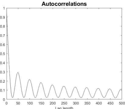
and is asymmetric about zero such as shown in Figure1.
Figure 1: ACF of a process with both an ARFIMA and a GARMA component.
Due to its flexibility, the multiple frequency GARMA approach has proven
very useful for modeling many physical, economic, and financial time series that
exhibit complex long memory features. Chung (1996b) estimates a single factor
model for sunspots andWoodward et al.(1998) andDiongue and Ndongo(2016)
provide evidence supporting the existence of multiple sources of long memory
in atmospheric CO2 and river flows. In economics and finance, these methods
have been used to study interest rates (Ramachandran and Beaumont 2001;
Gil-Alanaa 2007; Asai et al. 2018), exchange rates (Smallwood and Norrbin 2006),
inflation (Caporale and Gil-Alana 2011;Peiris and Asai 2016), equity prices (Lu
and Guegan 2011;Caporale and Gil-Alana 2014) and unemployment (Gil-Alanaa
2007) among many others. The possibility of multiple sources of long memory was
illustrated recently byLeschinski and Sibbertsen (2019) who modeled California
electricity load data using 14 independent long memory components.
Despite the increasing interest in the multi-factor GARMA model, a unifying
estimation approach does not appear to exist. Only a handful of studies have
rele-vant differencing parameters and the positions of the spectral poles, known as
Gegenbauer frequencies. Almost all studies assume the positions of the
singular-ities are known (see, for example, and Caporale and Gil-Alana (2011)) or they
employ two-step procedures where the Gegenbauer frequencies are typically first
estimated by inspection of the periodogram (see, for example, Lu and Guegan
(2011) andAsai et al.(2018), amongst others). A major difficulty lies in the fact
that estimation of the parameters dictating the positions of the spectral poles
appears to be non-standard. Perhaps more importantly, the relevant parameter
space is closed for these Gegenbauer frequencies, and there may exist a
disconti-nuity in the distribution at the zero frequency (see,Chung(1996a)). Additionally,
maximum likelihood based estimators in the frequency domain use a discrete set
of parameters for the associated singularities. For these estimators, as argued by
Giraitis et al.(2001), a full set of distributional results may not exist.
For inference for the models considered here, we are unaware of any study
proposing a full set of distributional results for any estimator. For a single factor
model,Giraitis et al.(2001) establish consistency for the Whittle estimator of the
Gegenbauer frequency and provide normality results for the differencing
param-eter. Hidalgo and Soulier (2004) discuss the properties of the log-periodogram
based semi-parametric estimates of the memory parameters for a multi-factor
model where the Gegenbauer frequencies are obtained from inspection of the
peri-odogram. For time domain maximum likelihood-based estimators,Chung(1996a)
provided promising results for a constrained sum of squares (CSS) method for
a single factor model based on the observation that, for the true parameter
val-ues, the expectation of the approximate likelihood function is zero. Regrettably,
given the difficulties involved with the distributions of the estimates of the spectal
poles,Chung (1996a) was unable to provide a rigorous initial proof establishing
consistency, causing his results to be questioned byGiraitis et al.(2001).
CSS estimator provides a feasible and relatively simple method to obtain joint
estimation results for the GARMA parameters. Recently, Beaumont and
Small-wood(2019) provided a comprehensive simulation study that generally supports
the results of Chung (1996a) excepting the case of parameter estimation of the
Gegenbauer frequency when the true value is 0. Additionally, as the CSS
estima-tor admits a continuous set of possible Gegenbauer frequencies, Beaumont and
Smallwood (2019) show that the CSS method generally obtains a smaller bias
for this parameter relative to the Whittle based counterpart. In comparison to
an MCMC Whittle estimator, Diongue and Ndongo(2016) further demonstrate
that the CSS method is relatively efficient in estimating differencing parameters
for k-factor GARMA processes with infinite variance disturbances. Given these
promising simulation results, it is worthwhile to consider the properties of the
CSS estimator when applied to models with multiple Gegenbauer frequencies.
In this paper, we review the mulit-factor GARMA model and present the
CSS estimator for all model parameters. Further, we extend the proofs ofChung
(1996b) to obtain proposed distributional results, which show that the estimates
of the Gegenbauer frequencies are asymptotically independent of each other and
all other model parameters. Since we are unable to provide a rigorous consistency
proof for the estimators of the sprectral poles, we provide simulation evidence to
help validate the results. The simulation evidence, including additional results
inBeaumont and Smallwood(2019), demonstrates that the theory can typically
be reliably used to provide inference for the estimated parameters.
The rest of the paper is organized as follows. In the next section, we present
the details of the multi-factor GARMA model. We present the CSS estimator
and derive its properties in Section 3. In Section 4, we present Monte Carlo
evidence for the finite sample precision of the iterative CSS estimation method
that we propose. In Section 5, we show that the weekly trading volume of IBM
and draw conclusions in Section 6, and an appendix contains technical details.
2. Multiple Frequency Long Memory Processes
The multiple frequency GARMA model was originally discussed byGray et al.
(1989) and presented in greater detail by Woodward et al. (1998) who refer to
the model as a k-factor GARMA model. The model is
φ(L)
k
Y
i=1
1−2ηiL+L2λi(xt−µ) =θ(L)εt, (1)
whereφ(L) andθ(L) are polynomials in the lag operator L such that φ(z) = 0
andθ(z) = 0 have roots outside the unit circle,{εt}is a white noise disturbance
sequence,λi are differencing parameters, and theηiare the parameters describing
the periodic features of the process. The Gegenbauer polynomials (1−2ηiL+L2)λi
have a pair of complex roots with modulus one and expand to an infinite order
polynomial in L. When k = 1, we get the single frequency GARMA model
(Hosking 1981;Gray et al. 1989), and when, in addition,η= 1 the model further
reduces to an ARFIMA(p, d, q) model (Granger and Joyeux 1980;Hosking 1981)
where, in this context, d = 2λ. Finally, we get an ARIMA model when η = 1
andλ= 0.5, and an ARMA process when λ= 0.
Assuming that eachηi is distinct, the k-factor GARMA model is stationary if
λi <0.5 whenever |ηi|<1, andλi <0.25 when|ηi|= 1.The model is invertible
ifλi >−0.5 whenever|ηi|<1, and λi >−0.25 when |ηi|= 1. Proofs for these
results are available inWoodward et al.(1998).
For stationary cases, the moving average representation is,
(xt−µ) =
θ(L) φ(L)
k
Y
i=1
1−2ηiL+L2−λi εt, (2)
from which the spectral density function is obtained as
f(ω) = σ
2
2π
θ(e−iω)
φ(e−iω)
2Yk
j=1
{2 |cos(ω)−cos(υj)|}−2λj, ω∈[0, π] (3)
where υj = cos−1(ηj) are the Gegenbauer frequencies. The spectral density
function is unbounded at allυj ifλj >0 and vanishes there if λj <0.
The autocovariances for a k-factor GARMA model can be computed as
γj = 2
Z π
0
f(ω) cos(ωj)dω, (4)
where special attention must be given to the singularities in f(ω) as recently
discussed byMcElroy and Holan(2016). Convenient expressions forγj are largely
available for single frequency models only. For example, whenη= 1 andλ <0.25,
the autocorrelations exhibit hyperbolic decay as demonstrated by Granger and
Joyeux (1980) for fractional processes. For GARMA models, Chung (1996a)
shows that for large j, the autocorrelation function with |η| < 1 and λ < 0.5,
λ6= 0, can be approximated as ρj ≈Jcos(j υ)j2λ−1, where J does not depend
uponj. This expression makes clear the hyperbolically damped sinusoidal pattern
of the autocorrelation function of a stationary GARMA process with|η|<1.
In Figure 1, we illustrated a model that combines ARFIMA and GARMA
models, which is of particular interest for economic and financial applications.
This example used a two frequency model with parameters (η1, λ1) = (1,0.15)
and (η2, λ2) = (0.992,0.25). Note that the first frequency corresponds to an
unbounded spike at the origin of the spectrum, and the second frequency
corre-sponds to an unbounded spike at the frequencyυ2 = cos−1(0.992) = 0.1266
radi-ans, or 0.0201Hz, which is very close to the origin. The ACF clearly demonstrates
3. Estimation
Several estimation procedures have been proposed for the k-factor model.
A likelihood-based Whittle method was studied byGiraitis et al. (2001), while
Hidalgo and Soulier(2004) advocate a semi-parametric method for λi after the
Gegenbauer frequencies have been selected via maximization of the periodogram.
In the frequency domain, wavelet procedures have been analyzed byLu and
Gue-gan(2011), whileDissanayake et al. (2018) use a state-space approach that uses
associated Gegenbauer polynomials and the Kalman filter to obtain likelihood
based estimates. Within this literature, there is no study that offers complete
distributional results for estimation of both νi and associated differencing
pa-rameters.1 Our approach is to estimate the k-factor GARMA model using a
time domain parametric estimator that is asymptotically equivalent to maximum
likelihood estimation. Specifically, we generalize the CSS estimator described by
Chung and Baillie(1993) for fractional models and by Chung (1996a,b) for single
frequency GARMA models. The procedure simultaneously estimates all
param-eters, including the ARMA components. Furthermore, we propose an analytic
asymptotic distribution for all of the parameters of the model.
Rewriting the MA representation of the model (2) in its AR form yields,
φp(L)
θq(L) k
Y
i=1
1−2ηiL+L2λi(xt−µ) =εt, (5)
where p and q indicate the orders of the ARMA terms. If we assume that the
initializing disturbances are zero, then the maximization of the CSS function
is asymptotically equivalent to maximum likelihood estimation. Under the
addi-tional assumption that the disturbances,εt,are iid normal with varianceσ2,then
1For the single factor case,Giraitis et al.(2001) provide normality results forλ, but are only
able to establish consistency for the Whittle estimator ofν.
thep+q+ 2 + 2kparameters, Ψ =φ1,, . . . , φp,θ1, . . . , θq, µ, σ2, η1, λ1, . . . , ηk, λk,
can be estimated by maximizing the CSS function
L∗(Ψ) =−T
2 log(2π)− T
2 log(σ
2)
−2σ12
T
X
t=1
ε2t. (6)
Note that the normality assumption is used here only to justify the
construc-tion of the CSS funcconstruc-tion, and is not necessary for the asymptotic theory
pro-posed below. We require only that the {εt} are martingale differences with
re-spect to an increasing sequence of sigma-fields, Ft, such that, for some β > 0,
suptE(|εt|2+βkFt−1)<∞, almost surely, and E(ε2tkFt−1) =σ2, almost surely.2
3.1. Asymptotic Distributions
We extend the proofs of Chung (1996 a,b) to propose distributional theory
for the CSS estimator in (6). Our proofs use the observation that the expectation
of the score for the CSS function achieves a zero value for the true parameter
set. We argue that an initial consistency proof for our full set of estimators may
not be available. In particular, we argue that the distributional results forηi are
non-standard with a discontinuity occurring at ηi = 1. In this specific case, it
is not possible to constrain all parameters to lie in the interior of the parameter
space, an assumption that would typically be employed in consistency proofs (see,
for example,Andrews and Sun(2004)). Consequently, we use an extensive set of
simulations to help validate results.
To extend Chung (1996a) and Chung (1996b), we consider four cases. The
first case is for those models for which |ηi| < 1 for all i = 1, . . . , k. The second
case is for those models for which there exists a singleηi = 1, and|ηj|<1 for all
other frequencies. The third case is for those models for which there exists a value
2As recently discussed by Peiris and Asai(2016), an additional advantage of the CSS
ηi = −1, and |ηj|< 1 otherwise. The fourth case is for those models for which
there exists two values ηi and ηj such that ηi = 1 and ηj =−1, with |ηm| <1
otherwise. The first theorem establishes that the asymptotic information matrix
for the k-factor GARMA model is block diagonal.
Theorem 1 (Independence of δ and η∗). Let δ = (λ
1, ..., λk, φ′, θ′)′ and η∗ =
(η1, ...., ηk)′ be the parameters associated with the CSS function for the k-factor
GARMA model. The asymptotic distribution ofδ is independent ofη∗.
The proof of this theorem is given in the Appendix. The essential idea is to
establish the different rates of stochastic convergence for the elements ofδandη∗.
Note that no conditions are placed on the value ofηi relative to ηj, i6=j, so this
theorem holds for all four cases described above. Consequently, the asymptotic
distribution ofδ can be considered independently of η∗.
Theorem 2 yields the asymptotic distribution of the estimators ofδ and µ.
Theorem 2 (Asymptotic distributions ofδ and µ). Let δˆbe the CSS estimator ofδ for the stationary and invertible k-factor GARMA model. (Ifµis unknown, we add the restriction thatηi6= 1 for all i= 1, . . . , k.) Then,
√
T(ˆδ−δ) N(0, Iδ−1), (7)
where denotes the weak convergence of the random vectors δ,ˆ and where
Iδ
(k+p+q)×(k+p+q)
=
Iλ1 · · · Iλ1λk Iλ1,φ Iλ1,θ
..
. . .. ... ... ...
Iλ1λk · · · Iλk Iλk,φ Iλk,θ
Iλ1,φ · · · Iλk,φ Iφ Iφ,θ
Iλ1,θ · · · Iλk,θ Iφ,θ Iθ
. (8)
The elements of Iδare defined as follows,
Iλi = 2
π2
3 −πυi+υ
2
i
, i= 1, . . . , k (9a)
Iλiλj = 2
"
π2
3 −πυi+
υ2i +υj2 2
#
, υi > υj, (9b)
Iλiφj = 2
∞
X
l=0
φ∗lcos[(l+j)υi]
(l+j) , i= 1, . . . , k, j = 1, . . . , p (9c)
Iλiθm = 2
∞
X
l=0
θ∗lcos[(l+m)υi]
(l+m) , i= 1, . . . , k, m= 1, . . . , q (9d)
where φ∗
l and θl∗ denote the lth coefficients in the infinite order expansions of
φ−1(L) and θ−1(L), respectively. The submatrices I
φ, Iφ,θ and Iθ consist of
ele-ments that are the same as the corresponding submatrices of the usual information matrix of an ARMA model. Finally, letηi <1, i=1,....,k. For the CSS estimator
of the mean,µ,ˆ with |ηi|<1 for alli, we have,
√
T(ˆµ−µ) N(0,2πf(0)), (10)
where f(0) denotes the spectral density function evaluated at frequency ω = 0. Further, the distribution of µˆ is equivalent to the sample mean x¯.
The proof of this theorem is given in the Appendix. Theorem 3 is the central
result and proposes the asymptotic distribution ofη∗ for all of our four cases.
Theorem 3(Aysymptotic distribution ofη∗). Let ηˆ
1, . . . ,ηˆk be the CSS
estima-tors of η1, . . . , ηk, for a stationary and invertible k-factor GARMA model based
on a sample {Xt}, t= 1, . . . , T, with ηi 6=ηj, i 6=j. Without loss of generality,
order the elements of η∗ from smallest to largest. Then let I
η1 denote the
denote the indicator function that takes on the value 1 ifηk = 1 and 0 otherwise.
If λi 6= 0, i= 1, . . . , k, then,
T(ˆηi−ηi)
sin(υi)
λi
hR1
0 W2i−1−Iη1 dW2i−Iη1 −
R1
0 W2i−Iη1 dW2i−1−Iη1
i
hR1
0 W22i−1−Iη1(r)dr+
R1
0 W22i−Iη1(r)dr
i (11)
with|ηi|<1, where i= 1 +Iη1, . . . , k−Iηk and,
T2(ηb1+ 1) − 1
2λ1
R1 0
Rr
0 W1(s)ds
dW1(r)
R1 0
Rr
0 W1(s)ds
2
dr , if ηb1 =−1 (12)
T2(ˆηk−1)
1 2λk
R1 0
hRr
0 W2k−1−Iη1(s)ds
i
dW2k−1−Iη1(r)
R1 0
hRr
0 W2k−1−Iη1(s)ds
i2
dr
,if bηk= 1, (13)
whereW1, W2, ...., W2k−Iη1−Iηk, are2k−Iη1−Iηk independent Brownian motions.
The proof is given in the Appendix. An important result of this theorem
is the asymptotic independence of the values in the vector η∗. In addition, for
each ˆηi,the values ofλi andυienter the equation for the asymptotic distribution
proportionally, so one only needs the values of the stochastic integrals depicted
in Theorem 3 to calculate asymptotic confidence intervals. The values for these
integrals are reported inChung(1996a).
3.2. Estimation Algorithm
These theorems provide important practical information for designing an
ef-ficient estimator. We know that the asymptotic distributions of the ˆλi’s are not
independent of ARMA parameters. Also, the asymptotic distribution of ˆδ and
ˆ
η∗ are independent, but the elements of ˆδ are Op(T−1/2),whereas ˆη
i isOp(T−1)
if|ηi| < 1 and Op(T−2) if |ηi| = 1. These results suggest that the algorithm of
Woodward et al. (1998), which estimates ARMA parameters independently of
(ηi, λi), will produce inconsistent estimates. It would be more appropriate to use
an extension of Chung’s method (Chung 1996a,b) by conducting a grid search
overη∗ combined with a gradient method over δ.However, Monte Carlo
simula-tions indicate that the grid over the η’s must be very fine, since the likelihood
function has many local minima. A k-dimensional line search forηi coupled with
a gradient based search for δ would be computationally infeasible, unless the
parameter space is bounded in some way or a very coarse grid is used.
The computational complexity of an estimator for a k-factor GARMA model
can be better appreciated when we consider the step of recursively computing the
residuals for the CSS estimator. Theith Gegenbauer polynomial in the k-factor
GARMA model can be expanded as (Gray et al. 1989)
(1−2ηiz+z2)−λi =
∞
X
j=0
C(λi)
j (ηi) zj, Cj(λi)(ηi) =
[Xj/2]
l=0
(−1)l(2ηi)j−2l Γ (λi−l+j)
l! (j−2l)! Γ (λi)
,
(14)
where [j/2] is the integer part ofj/2. As Chung(1996a) notes, the best way to
calculate the coefficientsC(λi)
j is via the following recursion,
C(λi)
j (ηi) = 2ηi
λi−1
j + 1
C(λi)
j−1(ηi)−
2λi−1
j + 1
C(λi)
j−2(ηi), (15)
where C(λi)
0 (ηi) = 1 and C (λi)
1 (ηi) = 2λiηi. Under the assumption that ε0 =
ε−1 =. . .= 0,the residuals can be calculated recursively from the expression
φ(L)(xt−µ) = k
Y
i=1
t−1
X
j=0
C(λi)
j (ηi)Lj
θ(L)εt. (16)
The combination of the k-dimensional product over the above sums create most
of the computational burden.
To overcome computational issues, coupled with different rates of convergence
by Ramachandran and Beaumont (2001). First, through inspection of the
peri-odogram and estimation of individual GARMA models, we choosek and obtain
a grid of starting values for each element ofη∗. We use each set of starting values
in this grid to obtain estimates for the δ. Conditional on the estimated value, ˆ
δ, we then estimate the elements of η∗ using an unconstrained gradient based
search.3 Using the updated estimates of η∗, new estimates of δ are obtained,
which are then used to update the estimates ofη∗. This procedure continues for all combinations of starting values forηi. The final model results from the set of
parameters that produce the smallest sum of squared errors. Although
compu-tationally intensive, the use of this multi-step gradient based iterative algorithm
provides large gains in computational time relative to the full k-dimensional line
search forηi, while also guaranteeing a continuous parameter space.
4. Finite Sample Performance
In this section, we report simulation results that examine the finite sample
properties of the CSS estimation. We are interested in examining the bias in
the parameter estimates and in comparing the finite sample standard errors of
the parameter estimates with the asymptotic standard errors. Chung (1996a,b)
and Ramachandran and Beaumont (2001) have done extensive simulations for
the single frequency GARMA model, with the latter paying particular attention
to the parametric region whereηis close to one and λis close to one-half. Based
upon those results, we will use a sample size of 300, and we will concentrate on
two frequency models with parameter ranges that we believe are most relevant
for economic and financial applications. We pay particular attention to the mixed
ARFIMA/GARMA case.
3The search occurs over all theoretically plausible values ofη
i, only imposing a constraint to
insureηi 6= ηj, i6=j. All elements of ηi are estimated jointly, unless it suspected that there
exists a value|ηi|= 1, in which case this parameter is estimated separately at each iteration.
The simulation results are presented in Tables 1–4. The columns of each table
list the parameters of the simulated model and each block in the tables gives the
results for a specific parameterization. Throughout, we report the true parameter
values (TRUE), the mean and median biases (MEAN BIAS; MED. BIAS), along
with the root mean squared error, mean of the numerical standard errors, and
mean absolute deviations (RMSE, MNSE, MAD) based on 1000 replications. For
computational purposes, we use an iterative procedure to generate a large amount
of data before discarding all but the last 300 observations. On rare occasions, the
generated data do not take on the properties of a multiple frequency GARMA
model. For the 17000 generated series below, it was necessary to discard three.
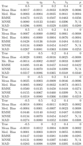
Table1presents the results for six different two frequency GARMA(0,0)
mod-els withηvalues of−12,0,21 andλvalues of 0.2 and 0.4.The estimation biases are
all quite small, especially for the η’s that converge at a faster rate than the λ’s.
Forλi, there is not much difference between the mean bias and the median bias or
the RMSE and the MAD, indicating that the distribution of these parameters is
quite robust. Generally speaking, a larger value ofλi mitigates the already small
bias inηi, which appears to be marginally more sensitive to estimation outliers.
This is likely due to the fact that an estimate ofλi near zero can lead to wildly
wrong estimates of the correspondingηi, since that Gegenbauer polynomial will
have very little impact on the likelihood function no matter what the value ofηi
is. In these cases, the mean,µ,is estimated with the sample mean, which is again
asymptotically equivalent to the CSS estimator ofµprovidedηi<1, i= 1, ..., k.
As noted above, the estimator for the mean is Op(T−1/2), the same rate of
con-vergence as the other parameters inδ, so its bias is also quite small.
To further validate the estimator, we compare the mean numerical standard
errors calculated from the estimated Hessian matrix in the last iteration with
the true asymptotic standard errors calculated with the aid of Theorem 2. In
Table 1: Simulations for the 2-factor GARMA(0,0) processes
η1 η2 λ1 λ2 µ
True 0.5 0 0.2 0.4 0
Mean Bias 0.0017 -0.0011 -0.0033 0.0029 0.0006 Med. Bias 0.0003 -0.0004 -0.0035 0.0041 0.0004
RMSE 0.0473 0.0155 0.0507 0.0463 0.0356
MNSE 0.0080 0.0133 0.0461 0.0396 N/A
MAD 0.0296 0.0091 0.0329 0.0395 0.0289
True 0.5 -0.5 0.2 0.4 0
Mean Bias 0.0007 -0.0000 -0.0002 0.0061 -0.0008 Med. Bias 0.0004 -0.0000 0.0004 0.0076 -0.0004
RMSE 0.0428 0.0136 0.0448 0.0484 0.0314
MNSE 0.0134 0.0069 0.0454 0.0457 N/A
MAD 0.0267 0.0081 0.0363 0.0388 0.0253
True 0 0.5 0.2 0.4 0
Mean Bias -0.0028 0.0001 -0.0016 0.0025 -0.0008 Me. Bias -0.0014 -0.0002 -0.0037 0.0033 0.0007
RMSE 0.0495 0.0146 0.0457 0.0442 0.0422
MNSE 0.0154 0.0070 0.0459 0.0399 N/A
MAD 0.0317 0.0086 0.0365 0.0348 0.0340
True 0 -0.5 0.2 0.4 0
Mean Bias 0.0025 0.0003 -0.0009 0.0046 -0.0006 Med. Bias 0.0005 0.0002 -0.0032 0.0073 -0.0015
RMSE 0.0500 0.0135 0.0458 0.0448 0.0274
MNSE 0.0155 0.0067 0.0460 0.0399 N/A
MAD 0.0318 0.0080 0.0366 0.0360 0.0219
True -0.5 0.5 0.2 0.4 0
Mean Bias -0.0018 0.0004 -0.0011 0.0025 0.0002 Med. Bias -0.0004 0.0001 -0.0007 0.0023 0.0008
RMSE 0.0446 0.0140 0.0442 0.0487 0.0383
MNSE 0.0134 0.0070 0.0454 0.0457 N/A
MAD 0.0274 0.0080 0.0352 0.0388 0.0308
True -0.5 0 0.2 0.4 0
Mean Bias -0.0010 0.0012 0.0004 0.0039 0.0002 Med. Bias 0.0001 0.0003 0.0019 0.0055 0.0003
RMSE 0.0447 0.0160 0.0381 0.0490 0.0285
MNSE 0.0131 0.0080 0.0397 0.0461 N/A
MAD 0.0283 0.0098 0.0299 0.0395 0.0228
the corresponding values of λ1 are 0.0394, 0.0450, 0.0394, 0.0455, 0.0450, and
0.0455, respectively. These values are quite comparable to the MNSE and RMSE
of the corresponding numbers in Table 1. The true asymptotic standard errors
for λ2 are 0.0455, 0.0450, 0.0455, 0.0394, 0.0450, and 0.0394, which again are
very close to their numerical counterparts. The true asymptotic standard errors
for the values of µare 0.0438, 0.0372, 0.0503, 0.0324, 0.0463, and 0.0351. Here,
the RMSE is comparable to the true asymptotic standard error, although it is
interesting to note that the RMSE slightly underestimates the standard deviation
of the mean in small samples. Finally, in light of the results of Theorem3, it is
not surprising to see that the MNSE and RMSE for the η’s are quite different,
since the RMSE assumes convergence at the rateT1/2.
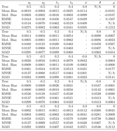
To examine the influence of the ARMA parameters, φ and θ, we choose a
particular parameterization (second case from Table1) and estimate various two
frequency GARMA(p, q) models with p and q being either zero or one. The
results are reported in Table2 and are similar to those in Table 1. Interestingly,
the main consequence of the inclusion of ARMA parameters is a relatively wide
distribution for the sample mean when a positive autoregressive parameter exists.
Again, for all of the cases considered in Table2, the median and mean biases are
Table 2: Simulation on the estimation of 2-factor GARMA processes with ARMA parameters
η1 η2 λ1 λ2 φ θ µ
True 0.5 -0.5 0.2 0.4 0.8 N/A 0
Mean Bias -0.0010 -0.0003 -0.0015 -0.0025 -0.0114 - -0.0101 Med. Bias 0.0003 -0.0002 -0.0016 0.0003 -0.0099 - -0.0107
RMSE 0.0444 0.0138 0.0456 0.0547 0.0429 - 0.1507
MNSE 0.0134 0.0070 0.0462 0.0519 0.0409 - N/A
MAD 0.0275 0.0082 0.0363 0.0441 0.0335 - 0.1212
True 0.5 -0.5 0.2 0.4 N/A 0.8 0
Mean Bias 0.0014 0.0003 -0.0011 0.0054 - -0.0099 -0.0007 Med. Bias 0.0005 -0.0001 -0.0011 0.0062 - -0.0086 -0.0023
RMSE 0.0488 0.0125 0.0480 0.0463 - 0.0459 0.0567
MNSE 0.0137 0.0068 0.0518 0.0463 - 0.0407 N/A
MAD 0.0295 0.0077 0.0389 0.0368 - 0.0362 0.0454
True 0.5 -0.5 0.2 0.4 -0.8 N/A 0
Mean Bias 0.0020 0.0016 0.0013 0.0078 0.0042 - 0.0004
Med. Bias 0.0009 0.0001 0.0011 0.0109 -0.0003 - -0.0000
RMSE 0.0461 0.0344 0.0516 0.0513 0.0431 - 0.0177
MNSE 0.0137 0.0068 0.0517 0.0464 0.0401 - N/A
MAD 0.0283 0.0089 0.0398 0.0381 0.0323 - 0.0141
True 0.5 -0.5 0.2 0.4 N/A -0.8 0
Mean Bias -0.0009 0.0009 -0.0026 0.0031 - 0.0167 -0.0001
Med. Bias 0.0000 0.0003 -0.0018 0.0058 - 0.0142 0.0001
RMSE 0.0526 0.0128 0.0457 0.0538 - 0.0539 0.0080
MNSE 0.0137 0.0070 0.0461 0.0521 - 0.0413 N/A
MAD 0.0299 0.0078 0.0364 0.0432 - 0.0413 0.0064
True 0.5 -0.5 0.2 0.4 0.8 0.8 0
Mean Bias 0.0002 0.0015 -0.0011 -0.0013 -0.0112 -0.0380 0.0045 Med. Bias 0.0003 0.0002 -0.0002 0.0016 -0.0041 -0.0281 0.0009
RMSE 0.0458 0.0221 0.0524 0.0578 0.0488 0.0739 0.2663
MNSE 0.0137 0.0069 0.0557 0.0548 0.0438 0.0467 N/A
MAD 0.0292 0.0083 0.0407 0.0442 0.0371 0.0546 0.2112
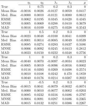
Table3examines the particularly interesting case whereη1=1 and η2 <1,so
that we get a combination ARFIMA and GARMA model. Compared toη2, the
estimator for η1= 1 has very little bias and extremely small RMSE and MNSE,
reflecting the fact that this parameter may beOp(T−2). The results for|η2|<1
are similar to those in Tables1and2, as are the results for theλ’s. Whenηi= 1,
however, the sample mean and CSS estimate of µ are no longer asymptotically
equivalent. Thus, we use the CSS estimator for the mean in these cases. The
computational difficulties of time domain estimators for ARFIMA models when
the mean is unknown have been well documented (Adenstedt 1974;Yajima 1991;
Chung and Baillie 1993;Cheung and Diebold 1994). In spite of these difficulties,
the mean is fairly unbiased, albeit with a wide distribution. Again, the remaining
[image:20.595.156.443.307.651.2]parameters suffer from very little distortion.
Table 3: Estimation of simulated ARFIMA/GARMA processes
η1 η2 λ1 λ2 µ
True 1 0.75 0.2 0.3 0
Mean Bias -0.0016 0.0026 -0.0127 0.0059 0.0417 Med. Bias -0.0000 0.0010 -0.0121 0.0080 0.0612
RMSE 0.0062 0.0195 0.0345 0.0420 0.4345
MNSE 0.0005 0.0069 0.0288 0.0410 0.3679
MAD 0.0016 0.0109 0.0275 0.0338 0.3543
True 1 0.5 0.2 0.3 0
Mean Bias -0.0023 0.0048 -0.0100 0.0041 0.0399 Med Bias -0.0001 0.0014 -0.0085 0.0049 0.0539
RMSE 0.0085 0.0274 0.0283 0.0437 0.3486
MNSE 0.0006 0.0092 0.0245 0.0413 0.2812
MAD 0.0023 0.0150 0.0222 0.0348 0.2756
True 1 0 0.2 0.3 0
Mean Bias -0.0040 0.0070 -0.0097 -0.0034 0.0023 Med. Bias -0.0005 0.0019 -0.0096 -0.0016 0.0002
RMSE 0.0116 0.0393 0.0269 0.0498 0.2574
MNSE 0.0010 0.0108 0.0242 0.470 0.1859
MAD 0.0040 0.0176 0.0214 0.0387 0.2022
True 1 -0.5 0.2 0.3 0
Mean Bias -0.0015 0.0041 -0.0079 -0.0032 -0.0074 Med. Bias 0.0000 0.0010 -0.0077 0.0002 -0.0203
RMSE 0.0085 0.0232 0.0316 0.0486 0.2797
MNSE 0.0004 0.0091 0.0287 0.0486 0.2365
MAD 0.0015 0.0132 0.0251 0.0386 0.2267
As noted above, the computational burden of the CSS estimator grows rapidly
we could narrow the range of the grid search, we could greatly improve the
efficiency of the algorithm. Withi6=j, sinceηi is independent of bothηj and the
parameters inδ, it may be possible to first estimate each value ofηi sequentially
to get good starting values. We could then re-estimate the entire model using
fairly tight grids over eachηi. In Table 4, we investigate this possibility. First,
we estimate a single frequency GARMA model and then filter the data with the
resulting Gegenbauer polynomial before estimating the second frequency using a
single frequency model on this filtered data. This process should produce good
[image:21.595.109.488.350.609.2]starting values for theη’s as long as the biases are not too large.
Table 4: Estimation of simulated ARFIMA/GARMA processes with single frequency models
η1 η2 λ1 λ2 φ θ µ
True 0.5 0.0 0.2 0.4 N/A N/A 0
Mean Bias 0.0099 0.0265 -0.0274 0.0487 - - 0.0006
Med. Bias 0.0023 0.0087 -0.0276 0.0535 - - 0.0007
RMSE 0.0603 0.0486 0.0468 0.0656 - - 0.0356
MNSE 0.0141 0.0473 0.0257 0.0103 - - N/A
MAD 0.0319 0.0279 0.0379 0.0566 - - 0.0285
True 0.5 -0.5 0.2 0.4 0.8 0.8 0
Mean Bias -0.0103 0.0027 -0.0975 -0.1278 -0.0796 0.0466 0.0045 Med. Bias 0.0159 0.0007 0.0971 -0.1256 -0.0752 0.0514 0.0009
RMSE 0.0787 0.0155 0.1010 0.1376 0.0955 0.0620 0.2663
MNSE 0.0202 0.0074 0.0374 0.0429 0.0481 0.0316 N/A
MAD 0.0406 0.0084 0.0975 0.1278 0.0814 0.0542 0.2112
True 1.0 0.75 -0.2 0.3 N/A N/A 0
Mean Bias -0.0019 -0.0151 0.0631 -0.1266 - - -0.0006
Med. Bias 0.0000 -0.0024 0.0611 -0.1254 - - -0.0008
RMSE 0.0336 0.0463 0.0689 0.1325 - - 0.0130
MNSE 0.0007 0.0085 0.0243 0.0302 - - N/A
MAD 0.0019 0.0143 0.0631 0.1275 - - 0.0105
The first two models in Table 4 are cases from the previous simulations,
and the third case represents a mixed ARFIMA/GARMA model in which the
ARFIMA component is short memory (λ < 0). The latter process may result
sidered in Table 4, the sample mean is used to estimate µ. We find that the
single frequency estimator generally first selects the frequency with the largest
corresponding value ofλ, thus capturing the most dominate feature of the
auto-correlation function. The results in Table4indicate that the small sample biases
inη1 and η2 are quite reasonable, suggesting that the method of choosing a tight
grid around these point estimates may work quite well. The relatively large biases
in the values of the vector δ, however, confirm the results of Theorem 2 that a
consistent estimator is obtained only through joint estimation of all parameters.
For a fixed sample size, these results strongly support the use of the
estima-tion algorithm, while largely validating the proposed distribuestima-tion theory.
No-tably, the distribution of ηi is independent of ηj, i 6= j, and the distribution
of these parameters is largely unaffected by the inclusion of ARMA dynamics.
Additionally, the proposed distribution theory for λi is confirmed. Finally, as
shown below, and in numerous other simulations that are available upon request,
the estimator achieves the proposed rates of convergence, even when we estimate
multiple GARMA components. This implies that confidence bands forηi will be
calculated in precisely the same way they are for the single frequency case, as
inChung(1996a). As such, any concerns that may exist regarding the proposed
distribution theory ofChung(1996a) will be inherited by the results here.
For the single frequency case,Chung(1996a) uses a line grid search to estimate
η, along with a gradient based method for δ. This implies that the parameter
space being searched over is a countable finite set that requires the use of
bound-ary constraints, given that a fine grid would be needed to capture an estimate of
η in the neighborhood of the true value. Based on the limited algorithm,Chung
(1996a) provides strong support for the proposed theory and associated
confi-dence bands for η for all cases except when η = 1. Here, it would appear that
the associated empirical sizes of tests forη= 1 under the null are too large to be
using a two-dimensional grid search over bothη andλwithout the use of
bound-ary constraints for η, and shows that the exact distributional results of Chung
(1996a) are generally supported, with two exceptions. First, similar to Chung
(1996a),Beaumont and Smallwood(2019) show the theory under the hypothesis
η = 1 is inappropriate for testing purposes. Confidence bands tend to be much
too wide, and empirical sizes are often much higher than their associated
the-oretical counterparts. Secondly, it is shown that with the use of the proposed
algorithm, the resulting empirical distribution has slightly fatter tails and a more
peaked density relative to the proposed theory. In terms of calculating confidence
bands, the issue appears to be very minor and disappears as the sample size
in-creases. Nonetheless, small biases in confidence bands can result, especially as
λapproaches 0. We now consider more complete simulation evidence to analyze
the extent to which these previous results carry over whenk >1.
For varying sample sizes, we considered a variety of parameterizations,
includ-ing models where there exists a value ofηi = 1. For brevity, the full set of results
are not reported here, but are available upon request. Here, we report only the
results for three fairly complicated 2-frequency parameterizations. Model 1 is a
GARMA(0,0) model with {η1, λ1} = {0.5,0.4}, and {η2, λ2} = {0,0.2}. Given
the distributional results above, this parameterization represents a case where
the process is expected to be especially volatile.4 Model 2 is also a GARMA(0,0)
model but with parameters {η1, λ1} ={0.98,0.45}, and {η2, λ2} = {−0.4,0.3}.
This parameterization approaches the region of the discontinuity in our
theo-retical distribution for η∗ and is also a strongly persistent process with λ 1 only
marginally less than 0.50. Model 3 is the same as Model 1 except we add an
AR(1) term with parameterφ= 0.80.
First, we compare the theoretical and simulated distributions of ηi. Figure2
4Note that the scaling factor in equation (11) of Theorem3is sin(νi)
λi so that, given a small
value forλ2 coupled withν2=π/2, the estimated value ofη2 is expected to be quite volatile.
Figure 2: Percentiles of theoretical and empirical CDFs for T=500 and T=2000.
shows the empirical and theoretical normalized cumulative distribution functions
(cdf) for η1 from Model 1 for sample sizes of 500 and 2000. For the empirical
distributions we plotT(ˆη−0.50) where the ˆη’s are computed using the estimation
algorithm described above, and the theoretical quantities have been calculated
using equation (11) from Theorem 3. The horizontal differences between the
theoretical and empirical curves show the disagreements between the theoretically
and empirically derived critical values for each percentile. The two horizontal
shaded regions show areas below the 0.025 and above the 0.975 percentiles, which
would be relevant for the construction of a 95% confidence interval.
The first observation is that the empirical and theoretical distributions are
in fairly close agreement, and this agreement is consistent as the sample size
increases. This suggests that the proposed convergence rate of T in Theorem 3
larger than implied by the theory, so we will now explore the consequences of any
such differences.
When estimating a multiple frequency GARMA model, the calculation of
confidence bands forηi is likely the most important application of the theory. To
get a sense of how applicable our proposed distribution theory and algorithm are,
Table 5 provides the estimated biases in calculating the upper and lower 68%,
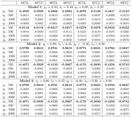
90%, 95%, and 99% confidence bands for the three models described above. As
a reference point, the theoretical bands for each value ofηi with a sample size of
500 are provided in bold font. Below the theoretical bands, we show the empirical
bands forη1 for each sample size, followed by the empirical bands forη2.
For Model 1, and with relatively small sample sizes of 500 observations, the
99% confidence bands are quite unreliable for η2 = 0. The theoretical
confi-dence band for η2 = 0 whenT = 500 is [−0.0423,0.0423], whereas, amongst the
5050 simulations, 99% of the estimated values of η2 were within a range from
−0.0423−0.0487 = −0.091 to 0.0423 + 0.026 = 0.068. In general, with small sample sizes, there are small but potentially non-negligible biases when using the
99% confidence bands. Otherwise, the results in Table 5 support the use of the
proposed distribution theory in calculating these intervals. First, we note that
the differences between the estimated and theoretical bands decrease sharply as
the sample size increases, and become negligible in most cases whenT = 2000.
Throughout, 68% and 90% bands are surprisingly accurate, such that multiple
confidence bands could be presented for researchers wishing to take a conservative
approach. Finally, we observe that there are no qualitative differences between
the estimated bands from the GARMA(0,0) and GARMA(1,0) models,
repre-sented as Model 2 and Model 3, suggesting that the values ofηi are independent
of ARMA components as implied by the proposed theory.
We also ran numerous simulations with η1 = 1, with results available upon
request, that match the findings inChung(1996a) andBeaumont and Smallwood
Table 5: Theoretical and empirical confidence intervals of theη’s
68%L 68%U 90%L 90%U 95%L 95%U 99%L 99%U
Model 1: η1 = 0.50,λ1= 0.40; η2= 0.00, λ2 = 0.20
η1: 500 0.4950 0.5050 0.4906 0.5094 0.4879 0.5120 0.4817 0.5183
ˆ
η1: 500 -0.0011 0.0011 0.0013 -0.0017 0.0030 -0.0037 0.0069 -0.0110
ˆ
η1: 1000 -0.0004 0.0007 0.0007 -0.0003 0.0017 -0.0013 0.0054 -0.0030
ˆ
η1: 2000 -0.0003 0.0002 0.0001 -0.0003 0.0005 -0.0008 0.0017 -0.0016
η2: 500 -0.0116 0.0116 -0.0217 0.0217 -0.0279 0.0279 -0.0423 0.0423
ˆ
η2: 500 0.0044 -0.0030 0.0157 -0.0111 0.0224 -0.0150 0.0487 -0.0260
ˆ
η2: 1000 0.0020 -0.0015 0.0069 -0.0053 0.0113 -0.0077 0.0203 -0.0128
ˆ
η2: 2000 0.0010 -0.0009 0.0034 -0.0030 0.0049 -0.0045 0.0103 -0.0076 Model 2: η1= 0.98, λ1 = 0.45;η2 =−0.40,λ2= 0.30
η1: 500 0.9790 0.9810 0.9781 0.9819 0.9775 0.9825 0.9763 0.9837
ˆ
η1: 500 -0.0003 0.0004 0.0000 0.0003 0.0003 0.0001 0.0011 -0.0004
ˆ
η1: 1000 -0.0001 0.0001 0.0000 0.0000 0.0001 -0.0001 0.0007 -0.0003
ˆ
η1: 2000 -0.0000 0.0000 0.0001 -0.0000 0.0001 -0.0001 0.0005 -0.0002
η2: 500 -0.4071 -0.3929 -0.4133 -0.3867 -0.4170 -0.3830 -0.4258 -0.3742
ˆ
η2: 500 -0.0004 -0.0002 0.0039 -0.0059 0.0072 -0.0092 0.0165 -0.0175
ˆ
η2: 1000 0.0001 -0.0002 0.0025 -0.0024 0.0047 -0.0042 0.0079 -0.0086
ˆ
η2: 2000 -0.0001 0.0000 0.0008 -0.0010 0.0019 -0.0018 -0.0048 -0.0042 Model 3: η1 = 0.98,λ1 = 0.45;η2 =−0.40, λ2 = 0.30,φ= 0.80
η1: 500 0.9790 0.9810 0.9781 0.9819 0.9775 0.9825 0.9763 0.9837
ˆ
η1: 500 -0.0002 0.0004 0.0003 0.0002 0.0009 -0.0001 0.0026 -0.0008
ˆ
η1: 1000 -0.0001 0.0001 0.0001 0.0001 0.0002 -0.0001 0.0010 -0.0004
ˆ
η1: 2000 -0.0001 0.0001 0.0001 -0.0000 0.0002 -0.0001 0.0004 -0.0004
η2: 500 -0.4071 -0.3929 -0.4133 -0.3867 -0.4170 -0.3830 -0.4258 -0.3742
ˆ
η2: 500 0.0008 0.0008 0.0060 -0.0045 0.0104 -0.0081 0.0250 -0.0158
ˆ
η2: 1000 0.0004 0.0001 0.0028 -0.0020 0.0049 -0.0032 0.0108 -0.0075
ˆ
η2: 2000 0.0002 0.0001 0.0013 -0.0010 0.0023 -0.0017 0.0048 -0.0038
(2019). The results show that the distribution theory under the nullη1 = 1 are
quite unreliable. In these cases, however,Beaumont and Smallwood(2019) argue
that more reliable results can likely be obtained by using the confidence bands
and testing procedures under the alternativeη <1, a suggestion we echo here.
5. Application
Emerging research has demonstrated that cyclical long memory is an
impor-tant characteristic of many financial time series.5 To demonstrate the
applica-bility of the CSS estimator and the proposed theory, we consider the weekly
trading volume of IBM equities measured in thousands from January 1, 1962
through July 1, 2019. Sequential estimation of single frequency models suggests
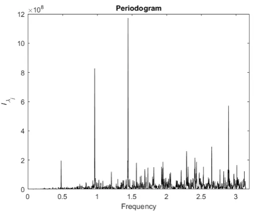
the strong possibility of at least 3 sources of long memory, and inspection of the
periodogram of the differenced series, which is depicted in Figure3, suggests up
to two more long memory frequencies.
We consider all combinations of k-factor GARMA(p,q) models with k ≤ 5
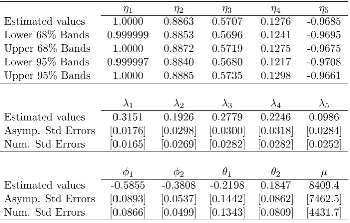
and p, q ≤ 2. Ultimately, a 5-factor GARMA(2,2) model was selected on the
basis of the Akaike information criteria, and the theory outlined above, where
all parameters are found to be statistically significant. Results are presented in
Table6. Based on the simulation results as discussed above, we show confidence
bands for the 68% and 95% quantities under the assumption that |ηi| < 1.6
Unambiguously, the results indicate that there potentially exists a singularity at
the origin, as all confidence bands contain the value 1 forη1.7
5See,Lu and Guegan(2011) andCaporale and Gil-Alana(2014) for recent applications to the
Nikkei-based forward premia and price dividend ratios associated with the S&P index. Also, see
Asai et al.(2018) who provide evidence of multiple sources of cyclical long memory in differenced interest rates for the US and Australia at various maturities.
6Recall that simulation results show that when η
i = 1, the confidence bands under the
alternative are more conservative and potentially more reliable than those under the null.
7Estimation results applied to the first difference of volume yield similar results. The
esti-mated value ofλ1is equal to -0.2114, which implies a value of 0.2886 for the series in levels. All other parameter estimates, which are available upon request, indicate no tangible disparities, including, most notably, the position of the spectral poles.
Table 6: Estimation of 5-frequency GARMA(2,2) model for IBM volume
η1 η2 η3 η4 η5
Estimated values 1.0000 0.8863 0.5707 0.1276 -0.9685 Lower 68% Bands 0.999999 0.8853 0.5696 0.1241 -0.9695 Upper 68% Bands 1.0000 0.8872 0.5719 0.1275 -0.9675 Lower 95% Bands 0.999997 0.8840 0.5680 0.1217 -0.9708 Upper 95% Bands 1.0000 0.8885 0.5735 0.1298 -0.9661
λ1 λ2 λ3 λ4 λ5
Estimated values 0.3151 0.1926 0.2779 0.2246 0.0986 Asymp. Std Errors [0.0176] [0.0298] [0.0300] [0.0318] [0.0284] Num. Std Errors [0.0165] [0.0269] [0.0282] [0.0282] [0.0252]
φ1 φ2 θ1 θ2 µ
Estimated values -0.5855 -0.3808 -0.2198 0.1847 8409.4 Asymp. Std Errors [0.0893] [0.0537] [0.1442] [0.0862] [7462.5] Num. Std Errors [0.0866] [0.0499] [0.1343] [0.0809] [4431.7]
Notes: Confidence bands are constructed assumingηi<1. Values in brackets are asymptotic
standard errors based on the estimated model, with ˆηi < 1, for all i using Theorem 2.
Figure 3: Periodogram of the first difference of IBM trading volume.
Given that the estimated values of the associated Gegenbauer frequencies,νi,
range from 0.0009 to 2.8898, we detect cycle lengths of 13.05, 6.52, 4.35, and 2.17
weeks, in addition to the extremely long, potentially infinite cycle associated with
a value ofη1 that cannot be distinguished from unity. To our knowledge, we are
the first to document the potential for multiple sources of long memory in equity
trading volumes, a finding that could be important in better understanding stock
market behavior.
6. Conclusions
In this paper we review the properties of a model that captures very diverse
patterns in the autocorrelation functions of data. The multiple frequency, or
k-factor, GARMA model generalizes existing long memory models and has the
particular advantage that the autocorrelations can decay at a non-monotonic rate
that is not necessarily symmetric about zero. In addition, the k-factor GARMA
Providing a full set of distributional results for estimators of k-factor GARMA
models has proven elusive. Building on the results inChung(1996a) and Chung
(1996b), we study a conditional sum of squares estimator and propose its
asymp-totic properties. The key feature of our results is that, for all possible values, the
asymptotic distribution ofηi is independent of all other parameters, including ηj
wheneveri6=j. It is important to note, however, that remaining parameters,
no-tably differencing parameters, are not asymptotically independent of each other,
and therefore methods that sequentially estimate these values will likely suffer
from severe bias. Finally, the model parameters are shown to converge at differing
rates. This greatly complicates attempts to establish rigorous initial consistency
proofs, especially given discontinuities in the distribution theory for ηi. We
at-tempt to overcome this shortcoming by conducting extensive simulations and
drawing on the recent work ofBeaumont and Smallwood(2019) to show that the
estimator performs in precisely the way our theory predicts in nearly all cases.
The simulation results show that the estimator performs well and that the
finite sample standard errors are close to the asymptotic calculations. In addition,
the simulation results suggest that the computational complexity associated with
a k-dimensional grid search can be greatly reduced via repeated estimation of a
single frequency GARMA model to obtain starting values. Further, the proposed
theory can be used to accurately obtain confidence bands for estimated values
of ηi. Finally, an application demonstrates the practical value of the k-factor
GARMA model. The trading volume of IBM is shown to be well modeled by a
five-frequency GARMA model with a spectral singularity at the origin.
Given the early success of multiple frequency GARMA models as discussed
in the introduction, our proposed estimator should find a number of important
applications in a myriad of fields. Further, the proposed distribution theory
will likely be useful in a number of contexts. For example, in instances where
sim-ulation results suggest that single factor models can be used to robustly select
Gegenbauer frequencies, thus complementing the use of methods based on
maxi-mization of the periodogram. Several challenges still remain. First, we are unable
to provide a rigorous initial consistency proof for our asymptotic results, which
we believe may prove quite elusive for the full model. However, it may be
pos-sible to consider a subset of Gegenbauer frequencies in this context. Perhaps
related, there appears to be some concern with the use of the proposed theory
when ηi = 1. Finally, computational difficulties may arise as the number of
fre-quencies, k, becomes large. Although our estimation procedures can limit this
problem by refining the grid for each ηi, recent research by Leschinski and
Sib-bertsen (2019) has identified cases where k could be as large as 14. It remains
to be seen if the resulting complexity would limit the practical implementation
of the CSS estimator for models that have a high number of spectral singularities.
Appendix
Proof of Theorem 1:
Consider the first order Taylor series expansion of the CSS estimators of
the invertible and stationary k-factor GARMA model of the process {xt}Tt=1
about the true parameter values δ = (λ1, . . . , λk, φ1, . . . , φp, θ1, . . . , θq) and η∗ =
(η1, . . . , ηk) :
1 √
T ∂L∗
∂δ
1
fT ⊙
∂L∗
∂η∗ + 1 T ∂
2L∗
∂δ ∂δ′ √1T F1T ⊙ ∂
2L∗
∂δ ∂η∗′
1 √
T
1
FT ⊙
∂2L∗
∂δ ∂η∗′
1 fT 1 fT ′
⊙ ∂2L∗
∂η∗∂η∗′
× √
T δˆ−δ
fT ⊙ ηˆ∗−η∗
=op(1) (A.1)
where⊙denotes element by element multiplication,fT and f1T denote k×1 vectors
whosejth elements are T and T1 when|ηj|<1 andT2 and T12 when |ηj|= 1. F1T
denotes the matrix formed by stacking the vector, f1
T
′
, on top of itself k times.
We will show that T1 ∂2L∗
∂δ ∂δ′ and
1 fT 1 fT ′
⊙ ∂2L∗
∂η∗∂η∗′,are Op(1),while
1 √
T
1
FT⊙
∂2L∗
∂δ ∂η∗′ possesses elements that are allop(1). Below, we show that the remaining
elements are bounded and find their proposed distribution. For largeT, we get
1 √
T σ2 PT
t=1εt∂ε∂δt
1
σ2f1T ⊙ PT
t=1εt∂η∂εt∗
+
Iδ
√ TF1
T ⊙Iδη∗
√ TF1
T ⊙ Iδη∗
1 σ2 1 fT 1 fT ′
⊙PTt=1 ∂
2ε
t
∂η∗∂η∗′
× √
T δˆ−δ
fT ⊙ ηˆ∗−η∗
=op(1). (A.2)
The cases forIφi,ηj, Iθi,ηj,andIλi,ηj when|ηj|= 1 follow from Chung (1996a,b).
UsingGradshteyn and Ryzhik (1980) equations 1.514 and 8.937.1, we find that
the information matrix elements ofIλi,ηj are
−E
1 T
∂2L∗
∂λi∂ηj
=E
"
4λj
σ2T
T X t=1 ∞ X l=1
cos(lυi)
l εt−l
! ∞ X
l=1
sin(lυj)
sin(υj)
εt−l
!#
. (A.3)
Under the assumptions governing εt, if υj > υi, and υi 6= υj, Gradshteyn and
Ryzhik(1980) equation 1.441.1 yields
Iλiηj =
2λj
sin(υj)
∞
X
l=1
sin[l(υi+υj)]
l +
∞
X
l=1
sin[l(υj −υi)]
l
!
= 2λj(π−υj) sin(υj)
. (A.4)
Thus, Iλiηj < ∞. If υj < υi, then the infinite sums in (A.4) are equal to
P∞
l=1
sin[l(υj−υi)+2πl]
l . FromGradshteyn and Ryzhik (1980) equation 1.444.1, we
see that the infinite sum converges. The same is true ifυi =υj.
If the remaining terms of all of the elements in (A.2) areOp(1) as shown below,
then the matrix in (A.2) is asymptotically block diagonal, and the distribution
of√T(ˆδ−δ) can be considered independently of fT (ηˆ−η) as claimed.
Proof of Theorem 2:.
are bounded, and the central limit theorem ofChan and Wei(1988),
√
T(ˆδ−δ) =−Iδ−1
"
1 √
T σ2
T X t=1 εt ∂εt ∂δ #
+op(1) N(0, Iδ−1). (A.5)
Information numbers for the diagonal terms of Iδ are given in Chung (1996a)
(page 251). The off diagonal terms,Iλiλj, which for large T and i6=j are,
−E
T−1 ∂
2L∗
∂λi∂λj
=E 1 T σ2
T
X
t=1
log(1−2ηiL+L2)εt log(1−2ηjL+L2)εt.
(A.6)
UsingGradshteyn and Ryzhik(1980) equations 1.514 and 1.443.3 yields,
Iλiλj = 2
∞
X
l=1
cos(l(υi+υj)) + cos(l(υi−υj))
l2 = 2
π2
3 −πυi+
υ2i +υj2 2
!
,
(A.7)
For the CSS estimator for ˆµ, the information number is:
Iµ=−E
T−1∂
2L∗
∂d2 µ = 1 σ2 φ(1) θ(1)
2Yk
i=1
(2−2ηi)2λi =
1 2πf(0)
−1, (A.8)
wheref(0) denotes the spectral density function evaluated at ω = 0. Now
con-sider the variance for ¯x. We have:
varh√T(¯x−µ)i= σ
2 T " T ( θ(1) φ(1)
2Yk
i=1
(2−2ηi)−λi
)#
= 2πf(0). (A.9)
By the central limit theorem of Chan and Wei, we also have √T(¯x −µ)
N(0,2πf(0)). The proof of the results forIλ1φj, Iλ1θm, . . . , Iλkφj,andIλkθmfollows
directly fromChung(1996b) in the single frequency case.
Proof of theorem 3:
Before proving Theorem 3 we state and prove the following useful lemma.
Lemma 1. Let ηˆ1, . . . ,ηˆk be the CSS estimators for η∗ = (η1, . . . , ηk) in a
tionary and invertible k-factor GARMA model. Then, withi6=j, 1
Tα
∂2L∗
∂ηi∂ηj
=op(1),
where α = 2 if |ηi|,|ηj|<1,{i, j ∈[1, k] : i6=j} (case 1), α = 3 if ηi =±1 and
|ηj|<1 (cases 2 and 3), and α= 4 if ηi=−1 and ηj = 1 (case 4).
Proof of the Lemma:
Case 1: |ηi|,|ηj|<1,{i, j ∈[1, k] :i6=j}. Without loss of generality, and
for ease of notation, rearrange the terms inη∗ such thatη
i =η1, ηj =η2. Let,
Zat=−
1 2λa
∂εt+1
∂ηa
= εt
(1−2ηaL+L2)
, a= 1,2. (A.10)
ApplyingGradshteyn and Ryzhik (1980) equation 8.937.1,
Zat=
1 sin(υa)
t
X
j=1
sin[(t+ 1)υa−jυa]εj,a= 1,2 (A.11)
which follows ifε0=ε−1 =....= 0. Now, define the random elements
ST(υa, r) =
√ 2 √
T σ2 [T r]
X
j=1
cos(jυa)εj,a= 1,2 (A.12a)
TT(υa, r) =
√ 2 √
T σ2 [T r]
X
j=1
sin(jυa)εj, a= 1,2 (A.12b)
where r ∈ [0,1] and [T r] is the integer part. Finally, from the expressions in
of trigonometry, we get the following expression,
4 sin(υ1) sin(υ2)
σ2
1 T2
TX−1
t=1
Z1tZ2t
= 1 T
TX−1
t=1
(cos[(t+ 1)ω2]−cos[(t+ 1)ω1])ST(υ1, t/T)ST(υ2, t/T)
−T1
TX−1
t=1
(sin[(t+ 1)ω1] + sin[(t+ 1)ω3])ST(υ2, t/T)TT(υ1, t/T)
−T1
TX−1
t=1
(sin[(t+ 1)ω1] + sin[(t+ 1)ω2])ST(υ1, t/T)TT(υ2, t/T)
+ 1 T
TX−1
t=1
(cos[(t+ 1)ω1] + cos[(t+ 1)ω2])TT(υ1, t/T)TT(υ2, t/T). (A.13)
Consider the random elements
Sn∗(υ1) =
n
X
j=1
cos(jυ1)εj and Tn∗(υ1) =
n
X
j=1
sin(jυ1)εj, (A.14)
and similarly for S∗
n(υ2) and Tn∗(υ2). Let{Xn}={Sn∗(υ1)Sn∗(υ2)}, and consider
the first term in (A.13). It is clear from the definition ofST(υ1,Tt) andST(υ2,Tt)
that T1 PTt=1−1cos[(t+ 1)ω2]ST(υ1, t/T)ST(υ2, t/T) =op(1) if
sup
1≤j≤T
j
X
n=1
einθXn
=op(T
2). (A.15)
First, observe that
E|Sn∗(υ1)Sn∗(υ2)| ≤ {ESn∗2(υ1)}1/2{ES∗2n (υ2)}1/2 ≤σ2n (A.16)
so thatE|S∗
n(υ1)Sn∗(υ2)|=O(n).Now let n≥m and consider
|Xn−Xm| ≤ |Sn∗(υ1)||Sn∗(υ2)−Sm∗(υ2)|+|Sm∗(υ2)||Sn∗(υ1)−Sm∗(υ1)|. (A.17)
Noting that
E|Sn∗(υ1)|2 =E(Sn∗(υ1))2 =σ2
n
X
j=1
cos(jυ1)
2
≤σ2n (A.18)
yieldsE|S∗
n(υ1)|2=O(n). Givenm≤n, this also impliesE|Sm∗(υ2)|2 ≤σ2n.
Next consider the expression
E|Sn∗(υ2)−Sm∗(υ2)|2 =σ2
n
X
j=m+1
cos2(jυ2)
≤σ2(n−m). (A.19)
Thus,E|S∗
n(υ2)−Sm∗ (υ2)|2=O(n−m).Similar reasoning implies thatE|Sn∗(υ1)−
S∗
m(υ1)|2 =O(n−m). Ifυ1 6=υ2, by Theorem 2.1 inChan and Wei (1988), we
see that the first term in (A.13) is op(1). By similar reasoning, the remaining
terms in (A.13) are also seen to be op(1). Thus, we have established that
4 sin(υ1) sin(υ2)
σ2
1 T2
TX−1
t=1
Z1tZ2t=op(1). (A.20)
This expression is asymptotically equivalent to
− 4λ1λ2 4 sin(υ1) sin(υ2)
4 sin(υ1) sin(υ2)
σ2
1 T2
TX−1
t=1
Z1tZ2t, (A.21)
which isop(1). So this completes the proof of Case 1 in the Lemma.
Case 2: Without loss of generality, letηk= 1, |ηj|<1, andj6=k.Rearrange
the polynomials inη∗ such thatηj =η1,and define the following elements,
Z1t=− 1
2λ1
∂εt+1
∂η1
= εt
(1−2η1L+L2)
,Z2t=− 1
2λk
∂εt+1
∂ηk
= εt
(1−L)2. (A.22)
Define the auxiliary process and its associated truncation.
Yt= (1−L)Z2t= t
X
j=1
This gives the following truncated series forZ2t,
Z2t= t
X
j=1
Yt= t
X
j=1
j εt−j+1. (A.24)
For ease of exposition, define the random process
XT(r) =
1 T
1 √
T σ
[T r]
X
j=1
Yj, (A.25)
and defineST(υ1, t/T) and TT(υ1, t/T) precisely as in (A.12). We then get,
√
2 sin(υ1)
σ2
1 T3
T−1
X
t=1
Z1tZ2t=
1 T
TX−1
t=1
sin[(t+ 1)υ1]ST(υ1, t/T)XT(t/T)
−T1
TX−1
t=1
cos[(t+ 1)υ1]TT(υ1, t/T)XT(t/T). (A.26)
Note that the expression
− √4λ1λk 2 sin(υ1)
√
2 sin(υ1)
σ2
1 T3
TX−1
t=1
Z1tZ2t, (A.27)
is asymptotically equivalent to T13 ∂ 2L∗
∂η1∂ηk. Define the processes
Sn∗(υ1) =
n
X
j=1
cos(jυ1)εj, Tn∗(υ1) =
n
X
j=1
sin(jυ1)εj, and Xn∗ = n
X
j=1
Yj, (A.28)
to facilitate the analysis. It is easy to verify that
1 T
TX−1
t=1
sin[(t+ 1)υ1]ST(υ1, t/T)XT(t/T) =op(1) (A.29)
if
TX−1
n=1
sin[(n+ 1)υ1]Sn∗(υ1)Xn∗ =op(n3). (A.30)
The same is true for the second term in (A.26). From (A.18) ES∗
n(υ1)2 ≤σ2n.
FromGradshteyn and Ryzhik(1980) equation 0.121.2, we have
EXn∗2 =E
n
X
j=1
j εt−j+1
2
=σ2
n
X
j=1
j2 =σ22n
3+ 3n2+n
6 ≤σ
2n3. (A.31)
Given, E|S∗
n(υ1)Xn∗| ≤ {ESn∗(υ1)2}1/2{EXn∗2}1/2, we see that E|Sn∗(υ1)Xn∗| is
O(n2).Now let n≥mand consider
|Sn∗(υ1)Xn∗−Sm∗(υ1)Xm∗| ≤ |Sn∗(υ1)||Xn∗−Xm∗|+|Xm∗||Sn∗(υ1)−S∗m(υ1)|. (A.32)
Clearly,E|S∗
n(υ1)|2 ≤σ2n, and from (A.19), E|Sn∗(υ1)−Sm∗(υ1)|2 ≤σ2(n−m).
From (A.31) we have,E|X∗
m|2 ≤σ3m3 ≤σ2n3. Finally, givenYj from (A.23),
E|X∗
n−Xm∗|2 =E
n
X
j=m+1
Yj
2
(A.33)
= (n−m)2
m
X
j=1
σ2+σ2
nX−m
j=1
j2 ≤σ2(n3−2n2m+n2m) =σ2{n2(n−m)}. (A.34)
Thus, from Theorem 2.1 inChan and Wei(1988),
sup
1≤j≤n
j X t=1
eitθSt∗Xt∗
=op(n
3) (A.35)
which implies that the first term in (A.26) isop(1). Following the same reasoning,
the second term in (A.26) is alsoop(1) and this proves Case 2 of the Lemma.
Case 3: Without loss of generality, let η1 =−1 and |ηj|<1, j 6= 1.
Rear-range the polynomials inη∗ such thatη
2 =ηj. Then,
Z1t=−
1 2λ1
∂εt+1
∂η1
= εt
(1 +L)2 =
t
X
j=1