Composite Quasi Likelihood Estimation of Dynamic Panels with Group Specific Heterogeneity and Spatially Dependent Errors

Munich Personal RePEc Archive

Composite Quasi-Likelihood Estimation

of Dynamic Panels with Group-Specific

Heterogeneity and Spatially Dependent

Errors

Chu, Ba

Carleton University

September 2017

Composite Quasi-Likelihood Estimation of Dynamic Panels

with Group-Specific Heterogeneity and Spatially Dependent

Errors

∗

Ba Chu

Carleton University

September 8, 2017

Abstract

This paper proposes a novel method to estimate large panel data error-correction mod-els with stationary/non-stationary covariates and spatially dependent errors, which allows for known/unknown group-specific patterns of slope heterogeneity. Analysis is based on composite quasi-likelihood (CQL) maximization which performs estimation and classification simultane-ously. The proposed CQL estimator remains unbiased in the presence of misspecification of the unobserved individual/group-specific fixed effects; therefore, neither instrumental variables nor bias corrections/reductions are required. This estimator also achieves the ‘oracle’ property as the estimation errors of group memberships have no effect on the asymptotic distributions of the group-specific slope parameters estimates. Classification and estimation involve a large-scale non-convex mixed-integer programming problem, which can then be solved via a new algorithm based on DC (Difference-of-Convex functions) programming - the DCA (DC Al-gorithm). Simulations confirm good finite-sample properties of the proposed estimator. An empirical application and a software package to implement this method are also provided.

Keywords: Large dynamic panels, Error-correction models (ECM), spatial dependence, common-group time variation (trends), mixing random fields, common-group-specific heterogeneity, clustering, composite quasi-likelihood (CQL), large-scale non-convex mixed-integer programs, difference of convex (d.c.) functions, DCA, K-means, Variable Neighborhood Search (VNS)

∗_{I gratefully acknowledge funding from the Social Science and Humanities Research Council of Canada (MBF} Grant 430-2016-00682).

1

Introduction

This paper proposes a novel method for estimation and inference of dynamic linear panel data models with unobserved group-specific patterns of slope heterogeneity and spatially dependent errors. Unobserved heterogeneity and spatial dependence across individuals/units have been the main focus of many econometric papers in panel data, and been well motivated from empirical economic problems, for example, in recent studies of empirical growth [see, e.g.,Durlauf, Johnson, and Temple (2005), Corrado, Martin, and Weeks (2005), Meliciani and Peracchi (2006), Alexiadis (2013),Durlauf and Quah (1999),Phillips and Sul (2007, 2009)]

A panel model with grouped heterogeneity in the slopes represents a viable approach to sum-marize grouped data as it is a compromise between a parsimonious model and another one with too many parameters. With data clustered in units, one can estimate three different models. In the first model, one can ignore the grouped structure in the units and estimate a regression with the data pooled. The estimates from this ‘pooled’ model will be biased if the units differ much, but with the pooled data, the model will become the most parsimonious in terms of the number of parameters estimated. At the other extreme, one could estimate one regression model for each unit, then take the average of all the estimated slope parameters if these parameters vary randomly around a constant - this approach is called the mean-group estimator [seePesaran and Smith(1995); Pesaran, Smith, and Im(1996) andFotheringham, Charlton, and Brunsdon.(1997)]. Pesaran, Shin, and Smith(1999) (PSS, henceforth) also propose the pooled mean group estimator for autoregres-sive distributed lag models (ARDL) that allow for both common parameters and heterogeneous parameters. However, this option produces way more parameters, and the estimates of the slope parameters will be highly variable if there are not many observations for each unit. The grouped slope heterogeneity approach represents a middle ground between these two extremes, thus it can be viewed as a compromise between completely ignoring the structure of the data and fully taking this structure into account by estimating many different models.

To be specific, a simple linear spatial-error specification with dynamic grouped patterns of heterogeneity takes the following form as a special case of a general ARDL model defined by (3.2) in Section 3:

∆yi,t =µi+φgi yi,t−1−θ

⊤

gixi,t

+λ∗_gi∆yi,t−1+δg∗i

⊤_∆x

i,t−1+ǫi,t, i= 1, . . . , N, t= 1, . . . , T, (1.1) where gi represents a group assignment that assigns each individual, i, to some specific group, say gi ∈ {1, . . . , G}; here G is the number of groups to be specified a priori; µi, i = 1, . . . , N, are individual-specific fixed effects; φgi, θgi, λ∗gi, and δ

∗

gi, i = 1, . . . , N, are common-group slope

space and time; for every given i ∈ {1, . . . , N}, ǫi,t are serially independent, and for every given

t_{∈ {}1, . . . , T_}, ǫi,t are spatially dependent [across locations], which effectively implies that ǫi,t and

ǫj,s, t6=s,are independent if i and j are associated with different locations - because ifǫi,t and ǫj,s are dependent, thenǫj,s and ǫj,t are also dependent asǫi,t are spatially dependent, this indeed leads to a contradiction.

As shown in Section4the proposed estimation procedure does not require any particular pattern of spatial dependence to be specified for the error terms; it merely assumes that the innovation terms

ǫi,t, i = 1, . . . , N and t = 1, . . . , T, are realizations of a centered, stationary mixing random field so that √Nǫ∗,t :=

√

N_N1 PN_i=1ǫi,t = √1_N PNi=1ǫi,t for t = 1, . . . , T can be approximated by serially independent Gaussian random variables under some mixing assumption on the random field ǫi,t as

N becomes sufficiently large, whence the composite quasi-likelihood (CQL) function can then be constructed. It is worth noting at this point that, in this estimation procedure, the normalized variance σ2

ǫ,N := N1V ar PN

i=1ǫi,t

of the spatial summation of errors and the cross-sectionally

average fixed effect µ_∗ := 1

N PN

i=1µi are treated as nuisance parameters. While µ∗ is estimated by

the maximum composite likelihood,σ2

ǫ,N can also be estimated directly by using robust (‘clustered’) standard errors formulas (see, e.g., Arellano (1987); Conley (1999); Driscoll and Kraay (1998); Kelejian and Prucha (2007)).

Heuristics

Since the parameters are common within each group, say g, the yi,t’s and xi,t’s of units within each group all have a common regression relationship, implying their common-group stochastic trends (namely time-varying sectional means) also do. Suppose that these time-varying cross-sectional means look quite distinct across groups (but similar within each group). To estimate the common slope parameters within each group,g, one could just regress the common-group stochastic trend of all ∆yi,t’s in this group on its lags and the common-group stochastic trends of all thexi,t’s in the same group and their lags. Since these common-group stochastic trends are unobservable, they can thus be proxied by common-group cross-sectional averages - this idea is inspired from the work by Pesaran (2006) which employs cross-sectional averages to provide valid inference in stationary panel regressions with a multifactor error structure. Importantly the regressions involving common-group cross-sectional averages do not induce an endogeneity problem which is often the consequence of doing the within-group or time-differencing transformations in dynamic panel data models. Thus the estimates will still be asymptotically unbiased even for T less than N. This intuition will be elucidated in Section4, and formalized in Section 5.

squared residuals amongst all the partitionings. However the number of regressions to run will be very large ifN is large (in fact, it is equal to a Sterling number of the second kind); this renders the so-called ‘many-regressions’ method infeasible. However, this method of running many regressions can be casted into a non-convex mixed integer programming problem as described in SectionC.1. Relation to the Existing Works

Hahn and Moon (2010) and Bester and Hansen (2016) show that the bias of grouped fixed effects (GFE) estimators asymptotically vanishes in nonlinear panel data models with finitely supported fixed effects (i.e., individual-specific fixed effects are common with each group, and differ across groups). The GFEs can be severely biased when individual-specific heterogeneity is incorrectly assumed to be constant within each group. Bonhomme, Lamadon, and Manresa’s (2016) method to discretize unobserved fixed effects can only reduce the bias of GFE estimators when the number of groups is allowed to grow with the number of individuals. Therefore, for the GFEs to be asymp-totically unbiased and normal when the number of groups is fixed, Bester and Hansen (2016) rely on the assumption that the maximum discrepancy between two individuals within groups goes to zero as the number of cross-sections becomes large.

In a typical dynamic linear panel, our proposed CQL estimator does not suffer from this type of bias arising due to misspecification of individual-specific heterogeneity because - unlike GFE estimators which require the individual/group-specific fixed effects to be concentrated out prior to estimation of the parameters of interest - the current estimation paradigm involves only the average fixed effect µ_∗ instead. Moreover, it is worth noting at this point that, since the within-group transformation in a linear dynamic panel gives rise to endogeneity, thus a least-squares estimator can be severely biased for small T, the proposed estimator does not rely on within-group transformation, thus it also does not suffer from an endogeneity bias. Therefore, instrumental variables (IV’s) or bias correction are not required to implement our method. In a dynamic panel with long time horizon the IV estimation strategy may not be feasible as the number of lagged variables that can be used as IV’s is large, thus another issue related to choice of optimal IV’s needs to be dealt with. Bias correction/reduction methods (see, e.g., Hahn and Kuersteiner (2002) and Dhaene and Jochmans (2015)) require preliminary estimators of the fixed effects to estimate the bias, thus a misspecification in the fixed effects can deteriorate the quality of bias estimates.

Works on panel data models with unknown patterns of group heterogeneity are pretty recent.1 Lin and Ng (2012) propose a conditional K-means procedure, which extends Forgy’s (1965) K-means algorithm, to estimate linear panel data models, but asymptotic theory is not derived. Bonhomme and Manresa(2015) [BM, henceforth] propose two minimum sum-of-squares clustering

algorithms based on the K-means algorithm and Hansen and Mladenovi´c’s (1997) Variable Neigh-borhood Search (VNS) algorithm to perform group classification and estimation in panels with time-variant grouped patterns of heterogeneity. In their asymptotic theory the GFE estimators are not influenced by the effect of group membership estimation because the probability of misclas-sifying at least one individual unit decays very fast as long as both N and T go to infinity such that N/Tδ _{↓ 0 for some δ > 0. When a lagged dependent variable is included as a covariate in a} model with additive time-invariant individual fixed-effects in addition to the time-varying grouped effects the infeasible fixed-effects estimator suffers from the incidental parameters problem (Nickell (1981)); IVs are then needed to produce consistent estimates for the parameters of interest. They also demonstrate that their proposed algorithms can achieve approximately the same optimal so-lutions to the least-squares clustering problem as other global optimizing algorithms (for example, the branch and bound algorithm) in panel datasets with a small number of groups.

Su, Shi, and Phillips (2016) [SSP, henceforth] propose a new variant of Tibshirani’s (1996) LASSO, namely classifier-LASSO, to perform group classification and estimation of regression slope coefficients simultaneously in a single step. However, this estimator often induces non-negligible asymptotic bias when it is applied to dynamic panels or panel regressions where some regressors are endogenous and the time horizonT is smaller, thus bias corrections of Hahn and Kuersteiner’s (2002) type are needed. Wang, Phillips, and Su (2016) propose a penalized least-squares criterion function using a new hybrid Panel-CARDS penalty function for simultaneous classification and estimation, effectively extending Ke, Fan, and Wu’s (2015) CARDS procedure for cross-sectional data to panel data.

Confidence bands for group memberships are derived in Dzemski and Okui (2017). Okui and Wang(2017) employBM’s clustering algorithm and group LASSO [see, e.g.,Chan, Yau, and Zhang (2014);Yuan and Lin (2006)] to estimate breaks and latent group structures in panels. Ando and Bai(2016) deal with linear panel data models with grouped factor structure and a large number of explanatory variables. The group membership of each individual can be estimated along with other parameters of the model. A LASSO approach is applied to select significant explanatory variables, and optimal group memberships can be found by using the K-means algorithm.

Nonlinear panel data models with discretized fixed effects are considered inBonhomme, Lamadon, and Manresa (2016). Druedahl, Jørgensen, and Kristensen (2016) consider a nonparametric GFE estimator for nonlinear panel data models with finitely supported fixed effects. Vogt and Linton (2017) develop methods to classify nonparametric regression functions into clusters based on the premise that there are groups of individuals who share the same regression function.

sum-of-squared-errors objective function. The proposed procedure is based on the premise that the response vari-ables and covariates for all units have non-zero common-group stochastic trends, thus it is natural to let the innovation terms of dynamic panel data models have some weak cross-sectional dependence that is summarized through a cardinality-based mixing coefficient [for mixing random fields] with polynomial decay rate. Due to the presence of these cross-sectionally dependent errors the growth rate of N relative to T that is required for the asymptotic normality and the ‘oracle’ property of the slope coefficient estimates will also depend on the degree of weak cross-sectional dependence. Computational Consideration

In the above-mentioned papers, various clustering techniques (notably, VNS with K-means inBM or classifier-LASSO inSSP) have been employed to partition panel data with latent group patterns while optimizing the associated objective function for estimates of group-specific coefficients. A common feature of these methods is that the problem is nonconvex and often nonsmooth (such as the K-means), thus falling into one of the most difficult areas of the optimization field. The proposed criterion function is also globally non-convex, and minimization of non-convex criterion functions of this type is a NP-hard (Non-deterministic and Polynomial-time hard) problem with possibly many local minima (Garey and Johnson,1979). Existing methods including the VNS and the K-means algorithm can feasibly search for ‘good’ local solution while exact solutions are often not known for large datasets with many individuals clustered into many groups; and the K-means often performs poorly when there are outliers in the data. So far the VNS using the K-means as a local search engine [as employed inBM] is still a common and effective strategy for data clustering especially when the number of groups is small.

Contributions

In light of the above discussions, we shall now summarize the main contributions. First, the proposed approach is motivated from an intuitive observation that common-group stochastic trends pertaining to the response and covariates can effectively identify common-group slope parameters. To estimate these common-group slope parameters and to select groups, one just needs to maximize a CQL function that pools up errors from regressions with unobserved common-group stochastic trends. This maximization problem has a novel form of a large-scale non-convex mixed-integer program, which can be written as a DC optimization problem. Given a starting point generated by the VNS, a DC algorithm with well-established convergence properties is then employed to maximize the CQL function. This optimization algorithm could be the most viable alternative to sequential procedures that iterate numerous large-scale convex optimization sub-problems [such as the algorithm inSSP], whose properties in computational complexity still remain open questions.

The second contribution sounds rather trivial, but it has an important implication for linear dynamic panels: Unlike conventional fixed effects or grouped fixed effects methods [that are often used to estimate dynamic panels], the proposed estimator is not subject to biases due to misspecifi-cation of the individual fixed effects as the form of fixed effects are completely irrelevant in the CQL function, and it is also asymptotically unbiased so that bias corrections are not required. These properties make the estimator appealing in this context whereas GFE estimators can be severely biased when individual fixed effects are in fact represented by a small number of unobserved types, and biases estimates can, as its consequence, be inconsistent.

Third, previous works on this topic do not cover the important issues of cross-sectional de-pendence and highly persistent covariates in panel regression models as the presence of either of these problems can have immediate consequences on inferential theory which is usually derived for the standard canonical case of cross-sectional independence and stationarity. This paper provides a unified approach to deal with all these issues of weak cross-sectional dependence and station-ary/nonstationary covariates. In all these scenarios, we show that, under some regularity conditions [which we will discuss in the main text], the proposed estimator maintains its ‘oracle’ property in the sense that the uniform convergence rates of the group memberships estimates are so fast that the estimates of the group-specific slope coefficients have the same asymptotic distributions as in the case with known group memberships.

cardinality-based mixing coefficient, and other tail probability inequalities, all of which can be useful for other applications as well. It is worth noting at this point that the proof of super-consistency for the group memberships estimates based on the VNS-DCA clustering makes use of an elegant duality between the penalized DC program on smooth polyhedral sets and the primal DC program with combinatorial constraints [as pointed out by (C.7) in the Supplemental Material] together with the Karush-Kuhn-Tucker (KKT) conditions for local optima.

Outline

The remaining of this paper is organized as follows. Section 3 introduces the model and main assumptions leading to the formulation of the maximum CQL estimation. Section 4 explains the main CQL estimation method for dynamic linear panel data models with group-specific heterogene-ity where the group structure can be left unspecified. The asymptotic properties of the proposed estimator together with a BIC-type information criterion used to select the optimal number of groups are all presented in Section5. When the covariates are stationary the estimates of the ‘true’ coefficients φ0,gi and θgi, i= 1, . . . , N, converge in distribution to normal random variables at rate

√

NT; this rate of convergence is the same as the rate that one could obtain when the parameters are homogenous, which is not a surprise as the number of groups remains fixed for any sufficiently largeN.

When the covariates are highly persistent the rate of the distributional convergence pertaining to the long-run coefficient θgi is T (instead of T

√

N as one may think of), which is essentially similar to the rate achieved with fixed N inPSS. This slow rate of convergence can be explained by the fact that, since the distributions of the response and covariates are not stable over time, one essentially needs more time-series observations for each individual when the number of cross-sections gets bigger in order to achieve a negligible classification error, which is then used to establish the ‘oracle’ property of the common-group slope parameters estimates. Derivation of the asymptotic theory is based on the premise that the spatial domainVN and the time horizon T grow to infinity jointly and the sample ratio |VN|/T depends on the polynomial decay rate of a cardinality-based mixing coefficient.

sizes and spatio-temporal error processes. Mathematical proofs of main theoretical results are collected in Section B in the Supplemental Material.

Finally, Section C in the Supplemental Material provides a detailed description of the main VNS-DCA algorithm and the derivations of the DC program used for clustering and estimation as an one-step procedure. It is important to note at this point that, since a standard DC program with mixed-integer sets can be transformed into an equivalent DC program with smooth polyhedral sets by employing a concave penalty function as in (C.7), the proposed CQL method can then be viewed as a penalty approach using some sort of combinatorial penalty function.

2

Notations

Some following conventional notations are commonly used: vectors/matrices and ‘sites’ on a sub-lattice (spatial domain) are written in boldface; _{k · k} denotes the Euclidean norm; A⊤ indicates the transpose of A; λmin(A) denotes the minimum eigenvalue of A; ιn is a n × 1 column vec-tor of ones and In is a n-dimensional [square] identity matrix; diag(A) denotes a diagonal ma-trix with A as the on-diagonal terms; for x,y _{∈ R}d_{, let < x,y > represent the scalar product} of x and y; |V| is the cardinality of a set, V; the Euclidean distance between two subsets, A

and B, is defined as d(A, B) := min{ka ₋ b_k : a _∈ A, b _∈ B}; the diameter of a set, A, is denoted by diam(A) := max_{ka ₋b_k : a,b _∈ A_}; Ac _{denotes the complement of a set, A;}

A_\B :=_{s: s_∈A and s_∈/ B_}; C0 represents a generic constant that may vary from one equation

to another; _⌊x_⌋ stands for the integer part of a (rational) number; 1(A) denotes a set characteristic function that takes value 1 ifAis true and 0 otherwise;_−→d ,_−→w ,and_−→p in order signify the distri-butional convergence, the weak convergence, and the convergence in probability; op(_·) andOp(·) are standard symbols for stochastic orders of magnitude; ‘w.p.1’ stands for ‘with probability approach-ing 1’;kXkγ := (E[|X|γ])1/γ denotes the H¨older norm; (a, b)+:= max(a, b) and (a, b)− := min(a, b); vec(A) denotes the vectorization of a matrix, A; and σ(per) _{: [1, G] → P ∈ P indicates a}

permu-tation operator that maps the set of original group labels, [1, G], to some set, P, in the collection of all sets of permuted group labels P. Also, to facilitate the reading of this paper, mathematical symbols (that are often referred to in the main text and the Supplemental Material) together with the places where they first appear are tabulated below.

ǫ_∗,t(Θ) composite errors with known group memberships, first defined in (4.1)

U |{z} G×N

:= (ui,c)∈RG×N a matrix of group membership indicators, first defined right below (4.9)

∆S a (G₋1)-dimensional simplex in RG, first defined right above (4.10)

g_∗,c := |VN,c_N | ∈(0,1) for c= 1, . . . , G group sizes, first defined right above (4.1)

ǫ_∗,t(Θ,U) composite errors with unknown group memberships,U,

first defined in (4.10)

ǫ∗,t(ψ,U) concentrated composite errors with unknown group

memberships, U, first defined in (4.12)

ξ_∗,t(θc) common-group cross-sectional mean of ξi,t, i =

1, . . . , N, in a known group, c, first defined right above

(4.1)

ξ_∗,t(θc,uc) common-group cross-sectional mean of ξi,t, i =

1, . . . , N, in an unknown group, c, first defined at the

beginning of Section 5.2

x(_∗c_,t) common-group cross-sectional means of xi,t, i = 1, . . . , N, in a known group, c, first defined in (4.4) x_∗,t(uc) common-group cross-sectional means of xi,t, i =

1, . . . , N, in an unknown group, c, first defined at the

beginning of Section 5.2

α(_·) the cardinality-based mixing coefficient for random fields, first mentioned in Definition B.1 in the Supple-mental Material

3

Model and Assumptions

Consider the following autoregressive distributed lag model for panel data observed on T time periods, t= 1, . . . , T, and N individuals (units),i= 1, . . . , N :

yi,t = p X

j=1

λgi,jyi,t−j+

q X

j=0

δ_g⊤_i,jxi,t−j +µi+ǫi,t, (3.1)

where the dx covariates (xi,t) and the p lags of yi,t (viz. yi,t−1, . . . , yi,t−p) are contemporaneously

uncorrelated with the errors ǫi,t; λgi,j for i = 1, . . . , N and j = 1, . . . , p and δgi,j for i = 1, . . . , N

are divided into G mutually exclusive, exhaustive groups; and the group membership variables

gi ∈ {1, . . . , G} are defined via an onto mapping g : {1, . . . , N} → {1, . . . , G}. To study the potential long-run relationship between yi,t and xi,t within each group, we shall rewrite (3.1) in the following error-correction form:

∆yi,t =µi+φgi(yi,t−1−θ⊤gixi,t) +

p−1

X

j=1

λ∗_gi,j∆yi,t−j + q−1

X

j=0

δ∗⊤_gi,j∆xi,t−j +ǫi,t, (3.2)

whereφgi := −

1−Ppj=1λgi,j

,θgi := −

Pq j=0δgi,j

φ_gi , λ∗gi,j :=−

Pp

m=j+1λgi,m forj = 1, . . . , p−1, and

δ_g∗_i,j :=₋Pq_m=j+1δgi,m for j = 1, . . . , q−1.

Suppose that each unit ,i, is associated with a location, say si, on a dv-dimensional Euclidean space, VN, equipped with the Euclidean metric k · k measuring the distance between any two locations in VN. Here, for clarity of exposition, VN is assumed to be a sublattice [of the standard

dv-dimensional integer lattice Zdv_{] indexed by N; the other cases where V}

N is some sublattice of

Rdv _{merely require a slight modification of the proofs with more notations as long as the distance}

between any two points in VN is greater than or equal to one (see, e.g., Jenish and Prucha(2012)). Random variables are spatially dependent at some point in time, t, if their measurements at two different locations depend on each other, and this dependence is assumed to be weaker as the distance between the locations becomes further. For the model to remain parsimonious and tractable, we can allow for spatial dependence in the relationship between y and x by assuming that, at a specific time period, the errorsǫi,t, i= 1, . . . , N andt= 1, . . . , T,at two different locations are dependent whilst they are independent at different points in time. First, we make the following assumptions:

Assumption 1 The errors, ǫi,t with i= 1, . . . , N and t = 1, . . . , T, defined in (3.2), are

indepen-dent across time and, at some given point in time, they are depenindepen-dent across locations such that ǫi,t ∼N(0, σi).

It is important to note that the normality of cross-sectional error terms, ǫsi,t, i = 1, . . . , N, in

Assumption 1 could be relaxed when N is sufficiently large since the CLT for strongly mixing random fields (see, e.g., Bulinski and Shashkin (2007)) warrants that _√1

N PN

i=1ǫi,t converges in distribution to a normal random variable (i.e., _√1

N PN

i=1ǫi,t for t = 1, . . . , T can be approximated by independent normal random variables.)

Assumption 2 The model (3.1) is stable in that the roots of

p X

lie outside the unit circle.

Assumption 2 is originally employed in PSS to ensure that the order of integration of yi,t is at most equal to the maximum of the orders of integration of the elements of the vector xi,t. This condition also warrants the existence of a long-run relationship between yi,t and xi,t within each group. Letwi,t := (∆yi,t−1, . . . ,∆yi,t−p+1,∆x⊤i,t, . . . ,∆x⊤i,t−q+1)⊤ denote a vector ofdw =p+dxq−1 auxiliary covariates, and let λgi := (λgi,1, . . . , λgi,p−1,δ⊤gi, . . . ,δ

⊤

gi,q−1)

⊤ _{be their coefficients. We can}

also rewrite (3.2) as

∆yi,t =µi+φgiξi,t(θgi) +λ⊤giwi,t +ǫi,t, (3.3)

where ξi,t(θgi) := yi,t−1−θ⊤gixi,t. Our objects for inference are the long-run coefficients θgi and the

long-run adjustment speed parameters φgi with i= 1, . . . , N.

It is important to note that, since the joint likelihood of the model is not the same as the product of likelihoods for each unit (or group), standard ML procedures will therefore involve a large un-known spatial variance-covariance matrix ofǫi,t, i= 1, . . . , N,thus they inevitably become infeasible. Moreover the expectations of the score functions of the concentrated joint log-likelihood function are not zero due to the absence of the complete orthogonality betweenǫi,t and ξi,t(θgi),thus

result-ing in significant biases. Therefore, here we shall instead construct the composite quasi-likelihood function. To simplify notations, we assume that the nuisance parameters are group-invariant (i.e., λg1 = · · ·λgN = λ.) Note that this simplification does not much change our mathematical

argu-ments, thus our asymptotic results will still remain valid even when these nuisance parameters vary over groups. To see this, notice that in the representation of the composite errors (4.3), the projec-tions ofx_∗,t’s and ξ_∗,t’s on the span of{w_∗,t : t= 1, . . . , T}can be of lower asymptotic orders when

T goes to infinity and the cluster sizes grow sufficiently large. In fact, simulation results reported in SectionA of the Supplemental Material confirm that the algorithm for clustering and estimation based on the objective function imposing group-invariant nuisance parameters performs well even when data are generated from a data generating process with group-variant nuisance parameters.

4

Estimation with Known/Unknown Group Memberships

theoretical properties, and behave well in many complex applications (see, e.g.,Reid (2013);Varin, Reid, and Firth (2011) for recent reviews of this subject matter.) Following Lindsay (1988), let

{f(y;θ), y _{∈ Y},θ _∈ Θ_}, where _{Y ⊂} Rn and Θ _⊂ Rd with n _≥ 1 and d _≥ 1, be a parametric model. Consider a set, _{A1, . . . ,Ak, . . . ,AK}, of marginal or conditional events associated with likelihoods, _Lk(θ;y) _∝ f(y _{∈ A}k;θ). A composite likelihood is formally defined as a weighted product QK_k=1Lk(θ;y)wk_{, where w}

k, k = 1, . . . , K, represent some non-negative composite weights

to be chosen.

We first present the main procedure based on composite quasi-likelihood to estimate Model (3.1) when group memberships of individuals/units are given (i.e., each individual belongs to a specified group.) By Assumption 1, √Nǫ_∗,t =

√

N 1

N PN

i=1ǫsi,t

i.i.d.

≈ N(0, σ2

ǫ), where σǫ2 := limN↑∞ N1V ar

PN i=1ǫsi,t

< _∞ if the spatial dependence among ǫi,t, i = 1, . . . , N, is weak for units that are far apart. Therefore, all the likelihoods associated with conditional events, _At(x) :=

{(ǫ1,t, . . . , ǫN,t)∈ RT :

√

N ǫ_∗,t =x} with t = 1, . . . , T, are approximately Gaussian, thus they are

referred to as quasi-likelihoods.

Let VN,c represent a set of locations for units in group c∈ {1, . . . , G} so that VN := SG_c=1VN,c,

LN,c := |VN,c|, and g∗,c := LN,c_N for c = 1, . . . , G. Define ∆y∗,t := _N1 PN_i=1∆yi,t, w∗,t := _N1 PN_i=1wi,t,

µ_∗ :=

( PG

c=1g∗,cµc if µ′is are group-specific,

1

N PN

i=1µi if µ′is are individual-specific,

and ξ_∗,t(θc) := _LN,c1 Pj∈VN,cξj,t(θc), where

µc := µg(VN,c) and θc := θg(VN,c), c = 1, . . . , G. Collecting all the unknown parameters into a

vec-tor, say Θ := θ⊤,φ⊤,λ⊤, µ_∗, where θ := θ₁⊤, . . . ,θ_g⊤, . . . ,θ⊤_G⊤ and φ := (φ1, . . . , φc, . . . , φG)⊤ with φc := φg(VN,c). Setting all the composite weights {wt, t = 1, . . . , T} to ones the composite

quasi-log-likelihood function (or composite quasi-likelihood function) can then be written as

QN,T(Θ, σǫ2) :=−

T

2 log 2π−

T

2 logσ

2

ǫ −

N

2σ2

ǫ T X

t=1

ǫ2

∗,t(Θ), (4.1)

whereǫ∗,t(Θ) := ∆y∗,t−µ∗−PGi=1g∗,iφiξ∗,t(θi)−λ⊤w∗,t.

Remark 4.1 Intuitively, while clustering with the least squares criterion function (as in _BM) is based on the premise that - for given values of the parameters - an individual is assigned to a group if its temporal summation of squared errors associated with that group is less than its temporal summations of squared errors associated with all other groups, the CQL criterion assigns a subset of individuals, sayC_{, to a group if the temporal summation of squared} C_{-mean errors (or centroids}

of any pair of groups are as little correlated as possible. To see this point, notice that 1 T T X t=1

ǫ2_∗,t(κ) = 1

T T X t=1 G X c=1 1 N N X i=1

ui,cǫi,t(κc) !2 = G X c=1 T X t=1 1 N N X i=1

ui,cǫi,t(κc) !2

| {z }

squared mean error of group c

+ G X c=1 G X

g6=c 1 T T X t=1 1 N N X i=1

ui,cǫi,t(κc) ! 1 N N X i=1

ui,gǫi,t(κg) !

| {z }

correlation between the mean errors of two groups ,

where κ = (κ⊤₁, . . . ,κ⊤_G)⊤_{. When groups are mutually independent, the CQL criterion function}

is the same as the summation of all the sums of squared errors obtained from G regressions of common-group stochastic trends.

To proceed, we concentrate out the nuisance parameters λ, and let Ω := (ψ⊤, σ2

ǫ)⊤ with ψ := (θ⊤,φ⊤, µ_∗)⊤. We can then obtain the concentrated composite quasi-log-likelihood function:

QN,T(Ω) :=−

T

2 log 2π−

T

2 logσ

2

ǫ −

N

2σ2

ǫ T X

t=1

ǫ2_∗,t(ψ), (4.2)

where

ǫ_∗,t(ψ) := ∆y_∗,t− T X

s=1

∆y_∗,sw_∗⊤,s ! _T

X

s=1

w_∗,sw_∗⊤,s !−1

w_∗,t

−

G X

c=1

g_∗,cφc 

ξ_∗,t(θc)₋ T X

s=1

ξ_∗(c_,s)(θc)w⊤_∗,s ! _T

X

s=1

w_∗,sw⊤_∗,s !−1

w_∗,t  

−µ_∗

 1−

T X

s=1

w_∗⊤_,s T X

s=1

w_∗,sw_∗⊤,s !−1

w_∗,t 

. (4.3)

To derive the first-order conditions for the CQL maximization, we first need to define the following quantities:

At |{z} Gdx×1

:= x(1)_∗,t⊤₋w⊤_∗,t T X

s=1

w_∗,sw_∗⊤,s !−1 _T

X

s=1

w_∗,sx(1)_∗,s

⊤

−w_∗⊤_,t T X

s=1

w_∗,sw_∗⊤,s

!−1 _T

X

s=1

w_∗,sx(_∗G,s)

⊤

!⊤

, (4.4)

where x(_∗c,t):= 1

LN,c X

j∈VN,c

xj,t for i= 1, . . . , G,

Bt(θ) | {z } G×1

:=  

T X

s=1

ξ_∗(1),s(θ1)w_∗⊤,s ! _T

X

s=1

w_∗,sw_∗⊤,s !−1

w_∗,t−ξ_∗(1),t(θ1), . . . ,

T X

s=1

ξ_∗(G_,s)(θG)w⊤_∗,s ! _T

X

s=1

w_∗,sw⊤_∗,s !−1

w_∗,t−ξ_∗(G,t)(θG)  

⊤

, (4.5)

and

Ct:= T X

s=1

w_∗⊤_,s T X

s=1

w_∗,sw_∗⊤,s !−1

w_∗,t−1. (4.6)

Some algebraic manipulations yield

∂QN,T(Ω)

∂θ =−diag(g∗,cφcIdx, c= 1, . . . , G)

N σ2

ǫ T X

t=1

ǫ_∗,t(ψ)At, (4.7)

∂QN,T(Ω)

∂φ =−diag(g∗,c, c= 1, . . . , G)

N σ2

ǫ T X

t=1

ǫ_∗,t(ψ)Bt(θ), (4.8)

and

∂QN,T(Ω)

∂µ_∗ =−

N σ2

ǫ T X

t=1

ǫ_∗,t(ψ)Ct. (4.9)

One can readily obtain the ‘oracle’ estimates ψe := θe,φe,µ_e∗ of the ‘true’ parameters ψ0 :=

(θ0,φ0, µ∗0) by finding the roots of (4.7)-(4.9).

Now we shall adapt the CQL procedure described above to the case where group memberships of individuals are not specified a priori. Suppose that the number of groups (or clusters)Gis given. Let U := (ui,c)_∈RG×N, i= 1, . . . , N and c= 1, . . . , G, be aG_×N matrix whose elements are defined by ui,c = 1 if individual i∈[1, N] belongs to group c∈[1, G], and ui,c = 0 otherwise. Because each individual can only be assigned to one group, we need to impose the constraint thatPG_c=1ui,c = 1 for everyi= 1, . . . , N.Moreover, let ∆S :=_{u_∈[0,1]G_: PG

c=1uc = 1}represent a (G−1)-simplex in RG, and ∆N

S indicates the Cartesian product of N simplices, ∆S; thus, U ∈ ∆NS T

With this matrix of group membership indicators, define the composite error as

ǫ_∗,t(Θ,U) := ∆y_∗,t−µ∗−λ⊤w∗,t− G X

c=1

1

N

N X

i=1

ui,cφcξi,t(θc). (4.10)

The CQL function is then given by

QN,T(θ,φ,λ, µ∗, σǫ2,U) := −

T

2 log 2π−

T

2 logσ

2

ǫ −

N

2σ2

ǫ T X

t=1

ǫ2_∗,t(Θ,U). (4.11)

By concentrating the nuisance parameters λ out, one readily obtains that

ǫ∗,t(ψ,U) := ∆y∗(w,t)− G X

c=1

1

N

N X

i=1

ui,cφc

y_i,t(w₋)₁−θ_c⊤x_i,t(w)₋µ∗1(tw), (4.12)

where

Z_t(w):= Zt− T X

t=1

Ztw_∗⊤,t ! _T

X

t=1

w_∗,tw⊤_∗,t !−1

w_∗,t

with Zt being either yi,t−1 orxi,t, and

1(tw):= 1− T X

t=1

w⊤_∗,t ! _T

X

t=1

w_∗,tw_∗⊤,t !−1

w_∗,t.

Moreover, notice that

∆y_∗(w_,t)= G X

c=1

1

N

N X

i=1

u0,i,cφ0,cξ(i,tw)(θ0,c) +µ∗01(tw),

where all the subscripts ‘0’ signify the true [unknown] quantities for the rest of the paper. The objective CQL functionQN,T defined by (4.11) is invariant with respect to all permutations of the group labels; let σ(per) _{: [1, G] → P ∈ P denote a permutation operator, which is a bijective}

mapping from the set, [1, G],of the original group labels to some set, P, of permuted group labels, and_P is the collection of all the sets of permuted group labels. It then follows that the concentrated composite error ǫ_∗,t(ψ,U) can also be written as

ǫ_∗,t(ψ,U) = G X

c=1

φ_σ(per)_(c)(θ_σ(per)_(c)−θ_0,c)

1

N

N X

i=1

u_i,σ(per)_(c)x(_i,tw)

+ G X

c=1

(φ0,c−φσ(per)_(c))

1

N

N X

i=1

+ G X

c=1

φ0,c 1

N

N X

i=1

(u0,i,c−ui,σ(per)_(c))ξ_i,t(w)(θ₀,c) +ǫ(₀w_,∗)_,t, (4.13)

whereǫ0,∗,t:= ǫ∗,t(Θ0,U0). The concentrated CQL function is then given by

QN,T(ψ, σǫ2,U) :=−

T

2 log 2π−

T

2 logσ

2

ǫ −

N

2σ2

ǫ T X

t=1

ǫ2_∗,t(ψ,U).

Consequentially, the maximum CQL estimates ψb, _bσ2

ǫ, and Ub of ψ0, σ2ǫ,0, and U0 respectively are

defined as the solutions to the following large-scale non-convex mixed-integer programming problem:

minnQN,T(ψ, σ2ǫ,U) : ψ∈Θψ ⊂RG(dx+1)+1, σǫ2 ∈Θσ ⊂R, and U ∈∆NS \

{0,1}G×No_{. (4.14)}

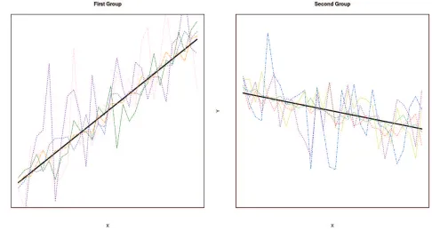
Intuition behind the proposed CQL estimator. Suppose that yi,t and xi,t share a common relationship in a group,c∈[1, . . . , G].The common-group stochastic trends that can be reasonably proxied by the observable vector of groupwise cross-sectional averages (y_∗(c,t),x

(c)

∗,t), c ∈ [1, . . . , G], also obey the same relationship, i.e., ∆y_∗(c,t) =µc+φcξ_∗(c,t)(θc) +λ⊤cw

(c)

∗,t+ǫ

(c)

∗,t.This point is illustrated in Figure1below. Since ǫ(_∗c_,t) will be close to zero as the group size is sufficiently large, one needs to blow it up by √N so that √NPG_c=1ǫ(_∗c_,t) _∼ N(0, σ2

ǫ). Therefore the CQL estimator can be viewed as the minimizer of the temporal average of the squares of the errors from regressions involving the common stochastic trends of yi,t and xi,t in G groups. For given N units, there are many ways to partition these N units into G groups. The estimated group memberships are associated with the group partitioning that minimizes the sum of squared residuals obtained from G regressions involving common-group stochastic trends.

5

Asymptotic Theory

5.1

Known Group Membership

First of all, it is important to note that the parameter spaces (Θθ, Θφ, Θµ, and Θσ) of (θ₀⊤,φ⊤₀, µ_∗0, σǫ,20)⊤

are assumed to be compact throughout the paper. We study the asymptotic behaviour of the ‘oracle’ estimateψein two different cases. In the first case, it is assumed that, for each i_∈VN, xi,t is a sta-tionary time series; and in addition the spatio-temporal processes {xj,t : j ∈ VN,c and t ∈ [1, T]},

c= 1, . . . , G,are mixing and satisfy the following assumption:

Assumption 3 Within each group, c, the random variables {xj,t : j ∈ VN,c and t ∈ [1, T]} are

Figure 1: Two groups of regression relationships with two different patterns of slopes. In all subplots: the bold dark line represents the exact relationship between common-group stochastic trends, yt(c) and x(_tc) with c= 1,2.

(a) the mixing coefficient - as represented by α(_·) in Definition B.1 [in the Supplemental Material] - for {(x(_tc), ǫj,t) : j _∈ VN,c and t ∈ [1, T]}, c = 1, . . . , G, where x(tc) are the

common-group stochastic trends of all the xj,t’s in group c, decays to zero at some rate such that

α(τ)≤Cθτ−θα for some

θα ≥max

p(dv + 1)γη (p−q)(γη−2)

+ (dv+ 1)γM,

dv+ 1 1_{− γ}2_η,

2p

p−4 −γM

!

,

where the generic constants Cθ >0, γη > 2, p > 4, q = _p2₋p₂, dv is the dimension of VN with

γM ≥1 provided in Definition B.1;

(b) maxj(E_kxj,1kp, Ekxj,1kγη, Ekxj,1k4)<∞;

(c) max_|VN|γMTγM+1−θα,|VN|γM(1−2/γη)Tǫ−1/2, T(γM+θα−1)ǫ−

1

2(θα−γM−1)|V_N|γM

↓ 0 for some ǫ _∈

0,min1₂, θα−γM−1

2(γM+θα−1)

.

Assumption 4 Let XN,T,t(θ) :=x(1)_∗,t⊤, . . . ,x(_∗G_,t)⊤,−ξ_∗(1),t(θ1), . . . ,−ξ_∗(G,t)(θG),−1 ⊤

ma-trix Dg

1

T PT

t=1Xt(θ0)Xt(θ0)⊤

D⊤_g, where Dg

|{z}

(G(dx+1)+1)×(G(dx+1)+1)

:= diag(g_⊗Idx,g,1) with g :=

(g_∗,1, . . . , g∗,G)⊤ ∈(0,1)G, is strictly positive.

A few remarks are now in order. Condition 3(a) imposes a specific degree of weak spatio-temporal dependence on the covariates and the error term. This type of cardinality-based mixing conditions is often used to quantify the notion of weak dependence in random fields, which includes time-series dependence as a special case (see, e.g., Doukhan (1994, Sec. 1.3.1) and also Bradley (2010) for an analytic treatment of various mixing conditions for random fields, including the mixing condition used in this paper).

It is important to note that, throughout this paper, we assume polynomial decay rates for the mixing coefficient for the reason that the mixing rate in stationary random fields is most of the time quite slow. Nevertheless, assuming the exponential rate can significantly simplify analytical arguments. As suggested in Bradley (1993) and Bradley (2007, Chap. 29) the mixing rate αs(τ) [in DefinitionB.1] can be of orderO(1/τ) or some arbitrarily slower rate. Many well-known spatial processes - including but not limited to linear fields (see, e.g., Guyon (1987)), the Cliff and Ord (1973) type spatial autoregressive processes using sparse spatial weight matrices, Volterra fields (see, e.g., Casti (1985)), and Markovian fields (see, e.g., Arbia (2006, Sec. 2.4.2)) - can verify this type of condition.

Condition 3(b) is rather standard - it requires some moments of the Euclidean norm of the vector of covariates to be bounded. Condition 3(c) allows both T and N go to infinity and the divergence speed of N relative to T depends on the structure of the spatio-temporal processes

{(x(_tc), ǫj,t) : j _∈ VN,c and t ∈ [1, T], c = 1, . . . , G, and the decay rate of the mixing coefficient. This condition is weaker than the condition [proposed in Hahn and Moon (2010)] that allows N

to be some exponential function of T (as such, N needs to be much greater than T) under some common types of weak serial dependence.

Assumption4is reminiscent of the standard assumption [employed in the OLS regression] about the positive-definiteness of the square matrix involving regressors. It basically requires that the covariates xi,t (or at least one of them) have non-zero cross-sectional means that may vary within each group, but these variations must be remarkably heterogeneous across groups. Therefore, if the probability limits of the common-group cross-sectional means g∗,cx(_∗c,t) = N1

PN

i=1u0,i,cxi,t,

c= 1, . . . , G,are similar across groups, or one of them is zero in some group, then this assumption

as well as the ‘well-separated groups’ assumption (Assumption 7below) become invalid. We now present the consistency ofψe for the stationarity case:

Theorem 1 (Consistency) Suppose that Assumptions1,2, 3, and4hold. Then,_|eσ2

ǫ−σǫ2|=op(1)

Theorem 2 (Asymptotic Normality) Let the conditions for Theorem 1 hold. Then,

√

NT(ψe₋ψ0)

d

−→σǫN 0,[Dφ0DgQzzDgDφ0]

−1

,

where Dφ

|{z}

(G(dx+1)+1)×(G(dx+1)+1)

:= diag(φ_⊗Idx,IG+1).

Remark 5.1 Since the CQL criterion function is nonlinear in the coefficientsθ andφof the error-correction representation defined via Eq. (3.2), it is not obvious to see the √NT-consistency of the CL estimators. To get some intuition about Theorem 2, we consider a linear panel data model with fixed effects and a group-specific slope coefficient: yi,t = µi +θgxi,t +ǫi,t for all i in group

g ∈[1,2, . . . , G]. Define µ_∗ := 1

N PN

i=1µi, xg := 1

T PT

t=1x (g)

∗,t, y := T1 PT

t=1y∗,t, zg := 1

T PT

t=1x (g)

∗,ty∗,t,

andxg,c := _T1 PTt=1x (g)

∗,tx

(c)

∗,t for g, c∈[1, G],where x

(c)

∗,t := N1 PN

i=1ui,cxi,t andy∗,t := _N1 PNi=1yi,t. The

‘oracle’ CQL estimate of ψ0 := (µ∗0, θ0,1, . . . , θ0,G)⊤ is given by

e ψ:=

 

1 x1 ··· xG

1 x1,1 ··· x1,G

..

. ... ... ...

1xG,1 ··· xG,G

 

−1" _y

z1 .. . zG # .

One can then obtain that:

√

NT ψe₋ψ0

=

 

1 x1 ··· xG

1 x1,1 ··· x1,G

... ... ... ...

1xG,1 ··· xG,G

 

| {z }

A

−1

   √N T PT t=1ǫ∗,t

√N T

PT t=1x

(1) ∗,tǫ∗,t

.. .

√N T

PT t=1x

(G) ∗,tǫ∗,t

  

, (5.1)

where ǫ_∗,t := _N1 PNi=1ǫi,t. Cross-sectional means can well approximate stochastic trends. Therefore,

by naively assuming xi,t to have an additive structure: xi,t = xg,t+xi with E[xi] = 0 for each

unit i in group g, one can obtain from law of large numbers that x_∗(g_,t) _≈ xg,t. Moreover, since ǫi,t

is a centered random error, we previously argued that √Nǫ_∗,t can be approximated by a normal

random variable, say Nt. By applying a central limit theorem, it then follows that q

N T

PT t=1ǫ∗,t

andqN T

PT t=1x

(g)

∗,tǫ∗,t, g = 1, . . . , G, can be approximated by mean-zero normal random variables as

long asx(_∗g,t) and ǫ∗,t are uncorrelated. The Gram matrix A can converge to a finite positive definite

matrix provided that xg,t, g = 1, . . . , G, are heterogeneous across groups. We can therefore obtain

the √NT-consistency. The same intuition carries over to general error-correction models.

Assumption 5 Let xi,t = Pts=1ηi,s, where ηi,s is a mixing centered spatio-temporal process; and

within each group, c _∈ [1, G], the random variables _{ηj,t, j ∈ VN,c and t ∈ [1, T]} are identically

distributed across space and time. Moreover,

(a) the mixing coefficient α(_·) for _{(ηj,t, ǫj,t) : j ∈ VN,c and t ∈ [1, T]}, c = 1, . . . , G, decays to

zero at a certain rate such that α(τ)_≤Cθτ−θα with some

θα ≥max

p(dv + 1)γη (p₋q)(γη−2)

+ (dv+ 1)γM,

dv+ 1 1₋ 2

γη

, 2p

p₋4 −γM

!

,

where the generic constants Cθ >0, γη >2, p > 4, q = _p2₋p₂, dv is the dimension of VN, and

γM ≥1 is provided in Definition B.1;

(b) maxj(E_kηj,1kp, Ekηj,1kγη, Ekηj,1k4)<∞;

(c) max_|VN|γMTγM+1−θα,|VN|γM(1−2/γη)Tǫ−1/2, T(γM+θα−1)ǫ−

1

2(θα−γM−1)|V_N|γM

↓ 0 for some ǫ _∈

0,min1₂, θα−γM−1

2(γM+θα−1)

.

Assumption 6 Let XN,T,t ≡ XN,T,t(θ0) be the same as in Assumption 4. It is assumed that the

minimum eigenvalue of the stochastic limiting matrix of the normalized Gram matrix:

Qzz :=plimN,T↑∞

(

diag T−1/2

IG×dx, N−

1/2

IG+1

Dg

N T

T X

t=1

XN,T,tXN,T,t⊤ !

×D_g⊤diag T−1/2IG×dx, N−

1/2

IG+1⊤

)

is positive.

A few remarks are now in order. It is worth noting that, when the covariates have common-group stochastic trends, say xi,t = x(tc)+

Pt

s=1ηi,s for every i ∈ VN,c with c= 1, . . . , G, the asymptotic

Theorem 3 (Consistency) Suppose that Assumptions 1, 2, 5, and 6 hold. Then, |σeǫ2 −σǫ,20| =

op(1), kθe−θ0k=op T−1/2

, _kφe₋φ0k=op N−1/2

, and _|eµ_∗−µ_∗0|=op N−1/2

.

To derive the limiting distribution of ψe, we define some further notations.

H(N,Tab)(φ) | {z } G×dx×G

:= diag(g_Idx)diag(φIdx)

(

N1/2

T3/2

T X

t=1

AtBt(θ0)⊤

)

diag(g),

H(N,Tac)(φ) | {z } G×dx×1

:= diag(g_Idx)diag(φIdx)

(

N1/2

T3/2

T X

t=1

AtCt )

,

H(N,Tbc) | {z } G×1

:= diag(g) (

1

T

T X

t=1

Bt(θ0)Ct )

,

H(N,Taa)(φ) | {z } G×dx×G×dx

:= diag(gIdx)diag(φIdx)

(

N T2

T X

t=1

AtA⊤t )

diag(gIdx)diag(φIdx),

and

H(N,Tbb) | {z } G×G

:= diag(g) (

1

T

T X

t=1

Bt(θ0)Bt(θ0)⊤

)

diag(g).

Let_HN,T(φ0) :=

 

H(N,Taa)(φ0) HN,T(ab)(φ0)H(N,Tac)(φ0)

H(N,Tab)(φ0)

⊤

H(N,Tbb) H

(bc)

N,T

H(N,Tac)(φ0) ⊤

H(N,Tbc)

⊤

1



.Lemma 5in the Supplemental Material effectively

implies that

lim

N,T↑∞HN,T(φ0) =H(φ0),

where_H(φ0) is a positive-definite stochastic matrix.

Theorem 4 (Asymptotic Normality) Let Assumptions 1, 2, 5, and 6 hold. Then,

  

T(θe₋θ0)

√

NT(φe₋φ0)

√

NT(µ_e∗−µ_∗0)

 

−→w MN 0,_H(φ0)−1,

5.2

Unknown Group Membership

We start by defining some common notations that will be used specifically for the rest of this section.

Letuc = (u1,c, . . . , uN,c)⊤ be a N×1 vector of group membership indicators associated with group

c ∈ [1, G]. In addition, with a slight abuse of notation, some of the symbols to be defined below may look the same as in Section5.1.

ξ_∗(w_,t)(uc)_≡ξ_∗(w_,t)(θ0,c,uc) := 1

N

N X

i=1

ui,cξi,t(w)(θ0,c), where ξi,t(w)(θc) :=y

(w)

i,t−1−θc⊤x

(w)

i,t ,

x(_∗w_,t)(uc) := 1

N

N X

i=1

ui,cx(i,tw),

ξ_∗(w_,t)(U, σ(per)_{) := ξ}(w)

∗,t (uσ(per)₍₁₎), . . . , ξ_∗(_,tw)(u_σ(per)_(G)) ⊤

,

x(_∗w_,t)(U, σ(per)) := x(_∗w_,t)⊤(u_σ(per)₍₁₎), . . . ,x_∗(w_,t)⊤(u_σ(per)_(G)) ⊤

,

Ft(U,U0) := x_∗(w,t)⊤(U,eσ(per)),ξ

(w)⊤

∗,t (U,eσ(per)),1

(w)

t ,ξ

(w)⊤

∗,t (U0, σ(per))−ξ_∗(w,t)⊤(U,σe(per)) ⊤

,

Dφ(_eσ(per)) := diag φσ_e(per)₍₁₎, . . . , φ_eσ(per)_(G)

,

θ(σ(per)) := θ⊤_σ(per)₍₁₎, . . . ,θ⊤_σ(per)_(G) ⊤

,

φ(σ(per)) := φσ(per)₍₁₎, . . . , φ_σ(per)_(G) ⊤

.

Therefore, in view of (4.13), one obtains that

ǫ_∗,t(ψ,U)₋ǫ(₀w_,∗)_,t =(θ(eσ(per))₋θ₀(σ(per)))⊤,(φ(₀σ(per))₋φ(σe(per)))⊤, µ_∗0−µ∗,φ(σ

(per)_)⊤

0

×diag Dφ(_eσ(per)),I2G+1

Ft(U,U0).

Moreover, let

H(Ub,U0) := max

σ(per)_∈σ(P)σe(permin)_∈σ(P)

1

N

G X

c=1

N X

i=1

|bu_i,eσ(per)_(c)−u_0,i,σ(per)_(c)|,

max

e

σ(per)_∈σ(P)σ(permin)_∈σ(P)

1

N

G X

c=1

N X

i=1

|bu_i,eσ(per)_(c)−u_0,i,σ(per)_(c)| !+

= min

e

σ(per)_∈σ(P)

1

N

G X

c=1

N X

i=1

|ubi,σe(per)_(c)−u_0,i,c|, min

σ(per)_∈σ(P)

1

N

G X

c=1

N X

i=1

|bui,c−u0,i,σ(per)_(c)| !+

,

where σ(_P) is the set of all permutation operators operating on _P, denote the optimal matching

H(ψb,ψ0) :=



 max

σ(per)_∈σ(P)σe(permin)_∈σ(P)

G X

c=1

bψ_eσ(per)_(c)−ψ_0,σ(per)_(c) 2 !1 2 , max e

σ(per)_∈σ(P)σ(permin)_∈σ(P)

G X

c=1

bψ_σe(per)_(c)−ψ_0,σ(per)_(c) 2 !1 2  + =   min e

σ(per)_∈σ(P)

G X

c=1

bψ_eσ(per)_(c)−ψ_0,c 2 !1 2 , min

σ(per)_∈σ(P)

G X

c=1

bψc−ψ0,σ(per)_(c) 2 !1 2  + ,

where ψbc := (θbc⊤,φbc,µb∗)⊤ and ψ0,c := (θ0⊤,c, φ0,c, µ∗0)⊤, be the optimal matching distance between

b

ψ and ψ0.

For the stationary case, we first need to state the following assumption:

Assumption 7 Suppose that limN_↑∞,T↑∞infH(U,U0)>ηuλmin

1

T PT

t=1Ft(U,U0)Ft(U,U0)⊤

> 0.

Moreover, let F_t(1)(U) :=x(_∗w_,t)⊤(U,_eσ(per)_),ξ(w)⊤

∗,t (U,eσ(per)),1

(w)

t ⊤

⊂Ft(U,U0), assume that

lim

N↑∞,T↑∞H(U,Uinf0)<ηu

λmin 1 T T X t=1

F_t(1)(U)F_t(1)⊤(U) !

>0.

Assumption 7states that groups must be well-separated in the sense that, if two matrices of group membership indicators, U and U0, are mismatched, then the Gram matrix involving differences,

ξ_∗(w_,t)⊤(U0, σ(per))−ξ_∗(w,t)⊤(U,eσ(per)),will be a positive-definite matrix. The second part of Assumption

7is similar to the standard assumption employed in the OLS regression.

Theorem 5 Under Assumptions 3, 4 and 7, it holds that √N H(ψb,ψ0)

p

−→ 0, H(Ub,U0)

p

−→ 0, and _|bσ2

ǫ −σǫ,20|

p

−→0.

Theorem6below gives the expected bias [in terms of theoptimal matching distance] of the estimates b

U(ψ) uniformly over allψ in a local neighborhood ofψ0.The rate at which this expected bias goes

to zero also depends on the decay rate of the mixing coefficient.

Theorem 6 Let {(x(_tc), ǫi,t) : i _∈ VN,c, t ∈ [1, T]} with c = 1, . . . , G represent a mixing

vector-valued spatio-temporal process and Ub(ψ) := argmin_U∈∆N S

T

{0,1}G×NN_T P_tT₌₁ǫ2_∗,t(ψ,U). Suppose that

(a) within each group, c _∈ [1, G], _{xi,t, ǫi,t}, i ∈ VN and t ∈ [1, T] are identically distributed over

time and space; (b) the mixing coefficient α(τ) < C0τ−θα, θα >

4γM

3 , 2dv+1

1−2/δα

+

for some δα > 2;

(c) kxi,tǫi,tk_δα < ∞; (d) maxjE[exp(ℓ|ǫj,t|)] ≤ Cℓ and maxjE[exp(ℓkxj,tk)] ≤ Cℓ for a positive

E

" sup ψ∈B(ψ0,ηψ)

HUb(ψ),U0

#

≤ C0

T−Cα _+N2γM _log2_(T)TγM−3₄θα _{+ exp}

−CM

T1/4

log2(T)

,

where B(ψ0, ηψ) is an open ball centered at ψ0 with an arbitrarily small radius, ηψ, in terms of the

optimal matching distance; and Cα and CM denote some sufficiently large constants that do not

depend on N or T.

Remark 5.2 It is important to note that most conditions in Theorem 6 above involve standard bounded moments and decay rates of the cardinality-based mixing coefficient, except Condition (d). The sub-exponential tails of ǫj,t andxj,t assumed there are needed to apply the truncation technique

that yields the first term T−Cα _{in the decay rate. The same condition is employed in Mammen,} Rothe, and Schienle (2012). This condition can be satisfied if the stationary density functions of ǫj,t and xj,t have compact supports.

In light of Theorem 6, we readily derive the decay rate of the optimal matching distance between the CQL estimatesψband the ‘oracle’ CQL estimates (i.e. the estimates constructed by maximizing the CQL function using the ‘true’ unknown groupsU0) ψe.The main result is stated in Theorem 7.

Again, this decay rate depends on the decay rate of the mixing coefficient.

Theorem 7 Let all the conditions in Theorem6 hold. Under Assumptions3, 4 and7, it holds that

Hψb,ψe=Op

NT−Cα_+NγM+1_log(T)TγM₂ −3₈θα _+Nexp

−CM

T1/4

log2(T)

,

where Cα and CM are some sufficiently large constants that do not depend on N or T.

Remark 5.3 Theorem 7 above shows that, if the mixing exponent θα is sufficiently large, the op-timal matching distance between the CQL estimate and the ‘oracle’ CQL estimate of ψ0 can decay

to zero faster than Op

1/√NT so that they are distributionally equivalent in the limit. From a practical point of view the availability of panel data permits the possibility of re-sampling each indi-vidual T times so that the probability of making a misclassification error is quite small even when N is quite large.

For the nonstationary case, let

ΛN,T(U,U0) := diag

r

N

T IG×dx,I2G+1

! 1

T

T X

t=1

Ft(U,U0)Ft(U,U0)⊤diag

r

N

T IG×dx,I2G+1

!

where the limit Λ(U,U0) is a stochastic matrix. We first state a variant of Assumption 7 about

group well-separability in Assumption 8below.

Assumption 8 lim infH(U,U0)>ηuΛ(U,U0)>0 for every ηu >0.

Theorem 8 Let xj,t =Pt_s=1ηj,s, where {(ηj,t, ǫj,t) : j ∈VN, t∈[1, T]} is a mixing vector-valued

spatio-temporal process. Suppose that (a) within each group, say c _∈ [1, G], _{ηi,t, ǫi,t}, i ∈ VN,c

and t _∈ [1, T] are identically distributed over space and time; (b) the mixing coefficient α(τ) < C0τ−θα, θα >

4γM

3 , 2dv+1

1−2/δα

+

for some δα > 2; (c) maxjkηj,tǫi,tk_δα < ∞; (d) (sub-exponential tails) maxjE[exp(ℓ_|ǫj,t|)]≤Cℓ andmaxjE[exp(ℓkηj,tk)]≤Cℓ for a positive constant, Cℓ>0, and

ℓ > 0 small enough; (e) N/T −→ const. Then, under Assumptions 1, 2, 5, and 8, it holds that

√

T Hθb,θ0

=op(1),

√

NHφb,φ0

=op(1), √N|µb_∗−µ_∗0|=op(1), and |bσǫ2−σǫ,20|=op(1).

Remark 5.4 Conditions (a) - (d) in Theorem8are similar to those in Theorem6, except Condition (e). This condition basically requires that N and T should grow at the same speed, or N must grow much more slowly than T while this growth rate of N relative to T is not needed in the stationary case. A simple explanation for this requirement is that, when covariates follow unit-root processes, a large number of time periods is needed to uncover a long-run relationship. Also, as the distributions of yi,t and xi,t are not stable, one may need in principle even more time-series observations when

the number of individuals gets bigger in order to achieve a negligible classification error.

Theorems9and 10below provide the decay rates for the expected uniform bias of the estimates of the ‘true’ group membership indicators, and for the optimal matching distance between the CQL estimates ψb and the ‘oracle’ CQL estimatesψe of ψ0.These theorems are the ‘nonstationary’

versions of Theorems6 and 7 (given above) respectively.

Theorem 9 Let Ub(ψ) := argmin_U∈∆N S

T

{0,1}G×NN_T P_tT₌₁ǫ2_∗,t(ψ,U). Suppose that the conditions of

Theorem 8 hold. Then,

E

"

sup

ψ_∈NN,T(ψ0,ηψ)

HUb(ψ),U₀

#

≤C0

(

N−Cα _+T−Cα_+N2γM _log2_(T)TγM−34θα+ exp −C_M T

1/4

log2(T)

!)

for some sufficiently large constants,Cα andCM,that do not depend onN orT,whereNN,T(ψ0, ηψ) :=T ηθ>0,ηφ>0,ηµ>0

(η2

θ+η2φ+η2µ)

1 2_=η

ψ

BT(θ0, ηθ)×BN(φ0, ηφ)×BN(µ∗0, ηµ)withBT(θ0, ηθ) :={θ ∈Θθ :

√

T H(θ,θ0)<

ηθ}, BN(φ0, ηφ) :={φ∈Θφ:

√

NH(φ,φ0)< ηφ}, and BN(µ∗0, ηµ) :={µ∗ ∈Θµ :

√

N_|µ_∗−µ_∗0|<

ηµ}.

Theorem 10 Assume all the conditions presented in Theorem9. Then, it holds under Assumption

Hdiag√TIG×dx,

√

NIG+1

b

ψ,diag√TIG×dx,

√

NIG+1

e ψ

=Op

N1−2Cα +N1/2T−Cα2 +NγM+12 log(T)TγM2 −38θα +N12 exp

−CM

T1/4

2 log2(T)

,

where Cα and CM are some sufficiently large constants that do not depend on N or T.

Empirical choice of the optimal number of groups. In the present maximum CQL paradigm, the optimal selection of the number of groups can be implemented by employing the following BIC-type information criterion. An information criterion is typically a sum of a goodness-of-fit measure and a penalty term used to account for the model complexity.

IC(G) := N

T

T X

t=1

ǫ2_∗,tψb,Ub+G_×ωN, (5.2)

where_|{z}Ub G×N

consists of CQL estimates for the ‘true’ group membership indicatorsU0given a number

of groups, G; ψb is the vector containing CQL estimates for the model parameters associated with the group classification provided byUb; both ψb and Ub are found by maximizing the CQL function in (4.11); and ωN is a penalty term that diverges with N at a certain rate (to be specified in Assumption 9 below).

Theorem11below suggests thatG∗ _{= argmin}

GIC(G) can consistently estimate the true number of groupsG0. To state this theorem, define some further notations.

XG,P,K,t(θ) :=



1(_tw), ξ(₀w_,∗)_,t(θ0,1), . . . , ξ0(w,∗),t(θ0,G),x_∗(w,t)(u0,1)⊤, . . . ,x(_∗w,t)(u0,P)⊤,ξt(w)(θ1)⊤

| {z }

1×N

, . . . ,ξ(_tw)(θK)⊤

 

⊤ ,

where ξ(_tw)(θ_c) := ξ₁(_,tw)(θ_c), . . . , ξ_N,t(w)(θ_c),

Z_G,P,t θ,U:= 1_t(w), ξ₀(w_,∗)_,t(θ_0,1), . . . , ξ₀(w_,∗)_,t(θ_0,G0),x_∗(w_,t)(u₁)⊤, . . . ,x_∗(w_,t)(u_G)⊤,ξ_t(w)(θ_0,1)⊤, . . . ,ξ_t(w)(θ_0,p)⊤,

ηP,t(θ)⊤

!⊤ ,

where ηP,t(θ) :=

(

ξ_t(w)(θ0,p+1)⊤, . . . ,ξt(w)(θ0,P)⊤⊤ if P ≤G0,

ξ_t(w)(θ_0,p+1)⊤, . . . ,ξ_t(w)(θ_0,G0)⊤,ξ_t(w)(θ_G0+1)⊤,ξ_t(w)(θ_P)⊤⊤ if P > G0;

ℓG,P,N,T :=

      

diag

1,IG0,

q

N

TIG×dx,IP×N

if P _≤G0,

diag

1,IG0,

q

N

TIG0×dx,IG×N,

1

TI(P−G0)×N

if P > G0;

X∗ (θ) := 1

T

X

where all of its elements converge in probability by the weak law of large numbers,

and

X∗∗G,P,N,T(θ,U) :=

1

T

T

X

t=1

ZG,P,t U,θZG,P,t U,θ⊤.

We also need the following assumption:

Assumption 9 Assume either of the following conditions:

(a) The vector of covariatesxi,t is stationary for eachi∈[1, N], and satisfies Assumption3. Also

the minimum eigenvalue of X∗N,T(θ) is strictly positive for every vector of pairwise different

sub-vectors, θ∗ := _{θ1, . . . ,θG}, as T and N become large. That is,

lim T,N↑∞G<Ginf

θ∗

λmin X∗G,N,T(θ∗)

>0,

where G is the maximum number of groups to cluster individuals.

(b) The covariates xi,t follow unit-root processes for each i ∈[1, N], and satisfies Assumption 5.

Besides, for every vector of pairwise different sub-vectors, θ⋄ := _{θG0+1, . . . ,θP}, and groups

with sizes that increase with N (i.e., limN↑∞ N1 PN