Count and duration time series with equal conditional stochastic and mean orders

Munich Personal RePEc Archive

Count and duration time series with

equal conditional stochastic and mean

orders

Aknouche, Abdelhakim and Francq, Christian

USTHB and Qassim University, CREST and University of Lille

11 November 2018

Online at

https://mpra.ub.uni-muenchen.de/97392/

Count and duration time series with equal conditional

stochastic and mean orders

Abdelhakim Aknouche

University of Science and Technology Houari Boumediene

and

Christian Francq

CREST and University of Lille

Abstract

We consider a positive-valued time series whose conditional distribution has a

time-varying mean, which may depend on exogenous variables. The main applications

con-cern count or duration data. Under a contraction condition on the mean function, it is

shown that stationarity and ergodicity hold when the mean and stochastic orders of the

conditional distribution are the same. The latter condition holds for the exponential

family parametrized by the mean, but also for many other distributions. We also

pro-vide conditions for the existence of marginal moments and for the geometric decay of the

beta-mixing coefficients. We give conditions for consistency and asymptotic normality

of the Exponential Quasi-Maximum Likelihood Estimator (QMLE) of the conditional

mean parameters. Simulation experiments and illustrations on series of stock market

volumes and of greenhouse gas concentrations show that the multiplicative-error form

of usual duration models deserves to be relaxed, as allowed in the present paper.

∗_{I am grateful to the Agence Nationale de la Recherche (ANR), which supported this work via the Project}

Keywords: Absolute regularity, Autoregressive Conditional Duration, Count

time series models, Distance correlation, Ergodicity, Exponential QMLE, Integer-valued

GARCH, Mixing.

1

Introduction

Models for nonnegative time series include the Autoregressive Conditional Duration (ACD)

model introduced by Engle and Russell (1998) to analyze durations between events (such

as trades, quotes, price changes), the Conditional AutoRegressive Range (CARR) model

introduced by Chou (2005) to study the range of an asset during a trading day, the more

general Multiplicative Error Model (MEM) introduced by Engle (2002) and count time

series models such as the INteger-valued AutoRegressive (INAR) studied by Al-Osh and

Alzaid (1987) or the Poisson INteger GARCH (INGARCH) studied by Ferland, Latour and

Oraichi (2006). Count time series models have been used in various domains, in particular

economics, finance, insurance, environmental science, social science and epidemiology (see

Davis, Holan, Lund and Ravishanker (2016) and the references therein). For MEM-like

mod-els, the stationary solutions are obtained explicitly, like for GARCH modmod-els, as function of

the parameters and the rescaled iid innovations of the model (see e.g. Francq and Zako¨ıan, 2019). INGARCH-type count time series models are not defined by means of an iid white

noise, but by assuming a discrete conditional distribution with a time-varying parameter

depending on the past values. Since the primary goal of these time series models is to

forecast the future level of the observed series, that parameter is generally the conditional

mean. The absence of an iid sequence in the definition of these models prevents exhibiting

an explicit solution. The fact that the support of the conditional distribution is countable

also prevents using the theory of Markov chains with continuous state space (see Meyn and

Tweedie, 2009). As a consequence, studying the probabilistic structure of most count time

series models is not obvious (see Fokianos, Rahbek and Tjøstheim, 2009, Tjøstheim, 2012,

stationarity results for INGARCH models with Poisson conditional distribution of linear

intensity parameter. Neumann (2011) proved the absolute regularity and relaxed the

linear-ity assumption on the Poisson intenslinear-ity parameter. Doukhan and Neumann (2019) showed

the absolute regularity for a much broader class of processes. Franke (2010) and Doukhan,

Fokianos and Tjøstheim (2012, 2013) studied the weak dependence of nonlinear Poisson

autoregressions. Douc, Doukhan and Moulines (2013) gave conditions on the associated

Markov kernel for stationarity and ergodicity of a first-order observation-driven time series

valued inN_{. These results have been extended to more general observation-driven models by}

Douc, Roueff and Sim (2015, 2016) and Sim, Douc and Roueff (2016). Gon¸calves,

Mendes-Lopes and Silva (2015) showed the stationarity and ergodicity of the INGARCH model with

compound Poisson conditional distributions. Davis and Liu (2016) showed stationarity and

mixing properties when the conditional distribution belongs to the one-parameter

exponen-tial family of distributions. The assumption that the conditional distribution belongs to

the exponential family is however restrictive. In particular, that assumption precludes the

zero-inflated distributions and hurdle models, which proved to be useful to deal with count

data sets that have an excess of zero counts (see e.g. Gurmu and Trivedi (1996), and Zhu (2012)).

The main aim of the present paper is to give stationarity and ergodicity conditions for

conditional distributions that are not restricted to belong to the one-parameter exponential

family. In addition we will allow the conditional mean to depend on covariates, which seems

relevant for some applications.

We thus consider a stochastic process of interest_{Yt, t∈Z}valued in the set [0,∞), and

a stochastic process of exogenous explanatory variables_{X_t, t_∈Z_{}valued in} Rr_{. LetFt be}

the information set available at time t, i.e. the sigma-field generated by _{Yu,Xu, u ≤ t}.

When there is no exogenous variable, i.e. when _Ft = σ(Yu, u ≤ t), the most frequent

specifications of λt :=E(Yt| Ft−1) is the linear equation

λt =ω+ q

X

i=1

αiYt−i+ p

X

j=1

where ω >0, αi ≥0 andβj ≥0. The standard ACD duration models and MEMs are of the

form

Yt=λtzt, (1.2)

where (λt) satisfies (1.1) and (zt) is an iid sequence of positive variables of mean 1, for

instance of exponential distribution of rate parameter 1. Note that for time series of counts,

i.e. when Yt is valued in N, the sequence zt = Yt/λt cannot be independent, in general.

Even for duration models for which the support of Yt is [0,∞), assuming that zt and λt

are independent is very restrictive. In particular, this implies that the conditional variance

Var(Yt | Ft−1) is proportional toλ2t, whatever the distribution ofzt. In the numerical part of

this paper, the independence betweenztandλtwill be assessed by bootstrapping the distance

covariance test of Sz´ekely, Rizzo and Bakirov (2007). For more versatile duration time series

models, it is thus of interest to relax the MEM specification (1.2), by only specifying a

conditional distribution with mean λt.

We refer to a distribution ofYtgivenFt−1 with mean (1.1) as a positive linear POLI(p, q)

model. If, as for INGARCH (p, q) models, the distribution ofYtgivenFt−1 is integer-valued,

the model is intended to represent time series of counts. If, as for the above-mentioned

extension of the ACD models, the distribution ofYtgivenFt−1 is valued in (0,∞), the POLI

model could suit for some time series of duration or volume, for instance.

Even if many references mention the possibility of adding exogenous variables in count

or duration time series models (see e.g. Cameron and Trivedi, 2001), we are only aware of few references focusing on exogenous variables: the paper on Poisson autoregresssion with

exogenous covariates (PARX) by Agosto, Cavaliere, Kristensen and Rahbek (2016) and that

of Liboschik, Fokianos and Fried (2017) which also considers negative binomial conditional

distributions and has the R companion package tscount (see also the R package acp of

Siakoulis, 2015). In the PARX model, we have

λt=ω+ q

X

i=1

αiYt−i+ p

X

j=1

βjλt−j+π⊤Xt−1, (1.3)

and π = (π1, . . . , πr)⊤ ≥0 componentwise. We also consider more general specifications of

the form

λt =g(Yt−1, . . . , Yt−q, λt−1, . . . , λt−p) +π(Xt−1), (1.4)

where the functions g and π are valued in [0,_∞).

We do not make a specific parametric assumption on the conditional distribution of Yt

given _Ft−1, but we assume that its stochastic order increases with its mean. More precisely,

let Fλ be a family of cumulative distribution functions (cdf) indexed by the mean λ =

R

ydFλ(y) ∈ R. Assume that, within this family, the stochastic order is equal to the mean

order, i.e.

λ_≤λ∗ _⇒ Fλ(y)≥Fλ∗(y), ∀y∈R. (1.5)

We shall refer to (1.5) as the stochastic-equal-mean order property. Section2gives examples

of cdf satisfying this property. Section3studies the existence and properties of a process (Yt)

with conditional meanλtand cdf satisfying (1.5). Subsection3.1assumes a linear conditional

mean of the form (1.3) and Subsection3.2 considers the more general specification (1.4). It

is shown that a positive-valued time series whose conditional cdf satisfies (1.5) and the mean

verifies mild regularity conditions is stationary and ergodic. When Yt is valued in N, we

show that the β-mixing coefficients have exponential decay rate. For some particular POLI

models, necessary and sufficient conditions for the existence of moments are also provided.

Section 4 considers the estimation of the parameters involved in the conditional mean λt.

Section 5 proposes a test of independence between zt and λt in the duration model (1.2).

Monte Carlo experiments and illustrations on series of trading volume and greenhouse gas

concentrations are presented. Concluding remarks are given in Section 6.

2

Examples of distributions with stochastic-equal-mean

order

We first recall that the exponential family is included in the class of the distributions for

that the conditional distribution of any ACD-MEM model also satisfies the

stochastic-equal-mean order property. We then give other examples of such conditional distributions which, to

our knowledge, are not yet fully considered in existing count or duration time series models.

2.1

One-parameter exponential family

Using Yu (2009), Davis and Liu (2016) demonstrated (see Proposition 6 and the discussion

after (2.1) in their paper) that (1.5) holds true when Fλ is the cdf of a one-parameter

exponential family on [0,∞). A distribution Fλ is said to belong to such an exponential

family if, with respect to a σ-finite measure, it admits a density of the form

gλ(y) = h(y) exp{ηy−A(η)}1{y≥0}, (2.1)

for some scalar natural parameterη=η(λ) and some twice differentiable cumulant

generat-ing functionA(η). It is known thatλ=A′_{(η). For exampleF}

λ can be the cdf of the Poisson

distribution with intensity parameter λ = eη_{. Recall that a random variable Y follows a}

negative binomial, Y ∼N B(r0, p0), of parametersr0 >0 and p0 ∈(0,1) if

P(Y =k) = Γ(k+r0)

k!Γ(r0)

pr0

0 (1−p0)k, k ∈N.

We have λ = r0(1−p0)/p0. This distribution also belongs to the exponential family when

p0 =r0/(λ+r0)) and r0 is fixed (withη = log(1−p0)).

2.2

Standard multiplicative ACD-type models

LetF_λ− be the quantile function associated to the cdf Fλ. Note that (1.5) is equivalent to

λ≤λ∗ ⇒ F_λ−(u)≤F_λ−∗(u), ∀u∈(0,1). (2.2)

By positive homogeneity of the quantile function, conditional on _Ft−1, the quantile function

of Yt satisfying (1.2) is

F_λ−_t(α) = λtF−(α),

whereF−_{is the quantile function ofz}

t. Therefore the conditional distribution of any standard

2.3

Additive duration models

An alternative to the multiplicative ACD model (1.2) is the additive model

Yt =λt−Eǫ1+ǫt, (2.3)

where (ǫt) is a stationary sequence of positive random variables, ǫt and λt are independent,

λt satisfies (1.3) or (1.4) with λt ≥ ω, and ω ≥ Eǫt to ensure positivity of λt. Any model

of this form satisfies (1.5) because Fλ(y) :=P(Yt ≤ y| λt =λ) =P(ǫ1 ≤y+Eǫ1 −λ) is a

decreasing function of λ.

2.4

Negative binomial NB

(

r

, p

)

with fixed

p

For any fixed p0, the negative binomial distribution Fλ with parameter r0 = p0λ/(1−p0)

apparently does not belong to the one-parameter exponential family. The next Lemma shows

that this family of distributions however satisfies (1.5). Write X _≤st Y when the random

variable Y stochastically dominates the random variable X, i.e. if P(X _≤ y) _≥P(Y _≤ y) for all y.

Lemma 2.1 If X _∼N B(r1, p0) and Y ∼N B(r2, p0) with r1 ≤r2, then X ≤st Y.

The previous lemma is quite obvious and can probably be found somewhere in the literature,

but we did not find a precise reference of such a result. For completeness, we thus give a

proof in Appendix.

2.5

Gamma distributions

A random variable Y is said to be Gamma distributed Γ(a, b) with shape parameter a >0

and rate parameter b > 0 if it admits the density g(y) = Γ−1_(a)ba_ya−1_e−by₁

{y>0}. We have

λ := EY = a/b. For fixed a, the distribution Γ(a, a/λ) readily belongs to the exponential

family (2.1). For fixedb, the distribution Γ(λb, b) is not of the form (2.1). However, denoting

by gλ(y) the density of that Γ(λb, b) distribution, it can be seen that when λ < λ∗ the

Ft−1 ∼Γ(λtb, b), then Var(Yt | Ft−1) =λt/b. This entails that (Yt) does not follow an ACD

model of the form (1.2), for which the variance is proportional to λ2_t.

2.6

Zero-inflated distributions

There exists numerous instances of count data sets with excess zeros with respect to a

baseline model, for example the Poisson distribution (see e.g. Ridout, Dem´etrio and Hinde (1998) and Zhu (2012)). One solution consists in assuming that a random element Y of the

data set has a zero-inflated Poisson (ZIP) distribution, given by

P(Y =k) =

  

τ + (1−τ)e−µ _{if k= 0}

(1₋τ)e−µ µk

k! if k >0.

(2.4)

Ifτ ∈[0,1], the ZIP(τ , µ) distribution (2.4) is that of a mixture of a proportionτ of variables

that structurally always take the zero value and a proportion 1₋τ of variables that follow

the Poisson distribution with intensity µ. When τ ∈[−e−µ_/(1−e−µ_{),0) and µ >0, the ZIP}

distribution is actually zero-deflated. The same law can be obtained with the hurdle model

which assumes that a proportionτ of variables always take the zero value and a proportion

1₋τ of variables follow the zero-truncated Poisson distribution

P(Y =k) =

  

τ if k = 0

(1−τ)e−µ_µk

(1−e−µ_)k! if k > 0.

More generally, assume that the baseline cdf is not necessarily Poisson _P(µ) but the cdf

Fλ, and define two zero-inflated distributions by

P(Y _≤y) = τ+ (1₋τ)Fλ(y), P(Y∗ ≤y) = τ+ (1−τ)Fλ∗(y), (2.5)

for all y _≥ 0 and P(Y _≤ y) = P(Y∗ _{≤ y) = 0 for all y < 0 , where τ ∈[0,1] is some extra}

zero probability. The following lemma shows that if the family of distributions Fλ satisfies

(1.5) then this is also the case for the zero-inflated distributions.

3

Probabilistic properties

We first consider the strict stationarity and ergodicity of the linear POLI-X model (1.3).

Ergodicity entails the strong law of large numbers, and is thus a fundamental tool for studying

the asymptotic properties of estimators and test statistics. We also discuss the existence

of moments in the case p = q = 1. We then extend the stationarity results for general

conditional means of the form (1.4), and show the geometric decay of the mixing coefficients

in the case where Yt is valued in N.

3.1

The linear conditional mean case

Theorem 3.1 Let _{Fλ, λ ∈ (0,∞)} be a family of cdf on [0,∞) (i.e. Fλ(y) = 0 for all

y <0) satisfying (1.5). There exists a stationary (and ergodic) sequence (Yt) such that

P (Yt≤y| Ft−1) = Fλt(y), (3.1)

where λt satisfies either (1.1) or (1.3) with (Xt) stationary and ergodic, if q

X

i=1

αi+ p

X

j=1

β_j <1. (3.2)

Conversely, if there exists a solution of (3.1) such that EYt =m < ∞, then Eπ⊤Xt <∞

and (3.2) holds.

Remark 3.1 (The exogenous variables do not matter for stationarity) The strict sta-tionarity condition (3.2) does not depend on the exogenous variables. This is not surprising since adding covariates remains to substitute a stationary interceptωt=ω+Pr_i=1πixi,t−1 for

the constantω in λt, and it is known (at least for conditional cdf belonging to the exponential

family) that the stationarity condition does not depend on the intercept. Francq and Thieu (2019) made a similar comment on GARCH models with exogenous variables.

Remark 3.2 (Markovian representation) The proof of Theorem3.1shows the existence of a solution of the form

where λt satisfies (1.1) or (1.3) with (3.2), Fλ satisfies (1.5), the sequences (Ut) and (Xt)

are independent and (Ut) is iid uniformly distributed in [0,1]. It follows that, given (Xt),

the process Z_t := (Yt−1, . . . , Yt−q, λt−1, . . . , λt−p)⊤ is a Markovian process. First note that

this excludes conditional means of AR(∞)-type λt = λ(Xt−1, Xt−2, . . .). This also suggests

using Markov chain techniques, as in Meyn and Tweedie (2009). However, when Yt is

integer-valued, those techniques seem difficult to apply. Note also that, in the case (1.1)with

p = q = 1, the conditional mean satisfies a Stochastic Recurrence Equation (SRE) of the form λt =ϕ(λt−1, Ut−1) where ϕ(λ, u) = ω+αFλ−(u) +βλ. It is also difficult to apply the

SRE theory, as developed in Bougerol (1993) and Straumann and Mikosch (2006), because the application λ 7→ F_λ−(u) is not continuous when Yt is integer-valued, and thus it seems

impossible to impose the Cauchy root test constraint

Elog sup

λ6=λ∗

|ϕ(λ, U1)−ϕ(λ∗, U1)|

|λ₋λ∗_| <0

required by the SRE theory (see Bougerol, 1993).

Remark 3.3 (Joint stationarity with the exogenous variables) The stationary solu-tion defined in the proof has a causal Bernoulli shift representasolu-tion of the form

Yt=ϕ(Ut, Ut−1, . . .;Xt−1,Xt−2, . . .).

It follows that, under the conditions of Theorem 3.1, the condition (3.2) also entails that the multivariate process (Yt,X⊤t )⊤ is stationary and ergodic.

Remark 3.4 (Link with the stationarity of ACD and GARCH) The square of a GARCH is an ACD model. It has been shown in Subsection 2.2 that any conditional distri-bution of an ACD model satisfies (1.5). Therefore, when Yt in Theorem 3.1 corresponds to

the square of a GARCH whose squared volatility λt follows (1.1), we retrieve the very well

From Theorem 3.1, we retrieve that (3.2) ensures the stationarity and ergodicity of the

Poisson-INGARCH(p, q) model (see Ferland, Latour and Oraichi, 2006) and of the NB(r0, pt

)-INGARCH(1,1) model withpt=r0/(λt+r0) (see Zhu (2011), Christou and Fokianos (2014)

and Davis and Liu (2016)). The theorem also provides new stationarity results, examples of

which are given in the following corollaries.

Corollary 3.1 (NB(rt, p0)-INGARCH) There exists a stationary and ergodic sequence

(Yt) such that the distribution of Yt conditional to Ft−1 is NB(p0λt/(1−p0), p0) where λt

satisfies either (1.1) or (1.3) with (X_t) stationary and ergodic if (3.2) holds.

Conversely, if there exists (Yt) such that Yt | Ft−1 ∼ N B(p0λt/(1−p0), p0) with EYt =

m <∞ and λt satisfies (1.3), then Eπ⊤Xt <∞ and (3.2) holds.

Corollary 3.1 is a direct consequence of Theorem 3.1 and Subsection 2.4. This result has

been conjectured by Aknouche, Bendjeddou and Touche (2018) but, to our knowledge, it

had not yet been formally proven.

We now consider a ZIP(τ , µ) distribution of the form (2.4). Zhu (2012) investigated such

conditional distributions with an INGARCH dynamics on the parameter µ. Denoting by λ

the mean of the ZIP(τ , µ) distribution, we have µ = λ/(1₋τ). To make the link between

Zhu (2012) and our framework, note that if τ is fixed and µ_t = ω +αYt−1 +βµt−1 then

λt = (1−τ)ω+ (1−τ)αYt−1 +βµt−1. Therefore, a linear dynamics on µt (as in Zhu 2012)

is equivalent to a linear dynamics on λt, under an appropriate change of notation. Since τ

is fixed, denote by FZIP

λ the cdf of the ZIP(τ , λ/(1−τ)) distribution.

Corollary 3.2 (ZIP) There exists a stationary and ergodic sequence (Yt) such that Yt |

Ft−1 ∼FλZIPt with τ ∈[0,1] andλt satisfies either (1.1) or (1.3), (Xt) being stationary and

ergodic, if (3.2) holds.

Conversely, if there exists (Yt) such that Yt | Ft−1 ∼ FλZIPt with EYt = m < ∞ and λt

satisfies (1.3), then Eπ⊤_X

t<∞ and (3.2) holds.

Corollary 3.2, which is a direct consequence of Theorem 3.1 and Subsection 2.6, shows the

stationar-ity under the same condition. The same results could be trivially obtained for zero-inflated

negative binomial conditional distributions.

We now give conditions for the existence of moments for the POLI(1,1) model. For

simplicity of notation, we write α and β instead of α1 and β1. Theorem 3.1 showed that,

for strict stationarity (and ergodicity), the precise form of the conditional distribution is

not important (provided it satisfies the stochastic-equal-mean order property (1.5)). For

the second-order stationarity, and more generally for the existence of moments, the next

proposition shows that the shape of the conditional distribution matters.

Theorem 3.2 Let _{Fλ, λ ∈ (0,∞)} be a family of cdf on [0,∞) satisfying (1.5).

As-sume that, for Y ∼ Fλ(y) and some integer ℓ ≥ 2, there exist nonnegative coefficients

aj(0), aj(1), . . . , aj(j) for all j ≤ℓ such that

EYj =

j

X

i=0

aj(i)λi for j = 1, . . . , ℓ. (3.3)

Under (3.2), let (Yt) be a stationary sequence such that P (Yt≤y| Ft−1) =Fλt(y), where λt

satisfies (1.1) with p=q = 1. We have EYℓ

t <∞ if and only if ℓ

X

j=0

a(j)

ℓ j

αjβℓ−j <1, (3.4)

where a(0) =a(1) = 1 and a(j) =aj(j) for j ≥2.

Example 3.1 (NB(r0, pt)) The first momentsmi =EYi ofY following the BN(r0, r0/(λ+r0))

distribution are

m1 = λ, m2 =λ+

1 +r0

r0

λ2, m3 =λ+ 3

1 +r0

r0

λ2+2 + 3r0+r

2 0

r2 0

λ3,

m4 = λ+ 7

1 +r0

r0

λ2 + 62 + 3r0+r

2 0

r2 0

λ3+ 6 + 11r0 + 6r

2 0+r03

r3 0

λ4.

It follows that (3.3) holds with

a(2) = 1 +r0

r0

, a(3) = 2 + 3r0+r

2 0

r2 0

, a(4) = 6 + 11r0+ 6r

2 0+r30

r3 0

Theorem 3.2 shows that the POLI(1,1) model with BN(r0, r0/(λt+r0)) conditional

distribu-tion admits a moment of

order 2 iff (α+β)2+α

2

r0

<1, (3.5)

order 3 iff (α+β)3+3α

2_(α+β)

r0

+2α

3

r2 0

<1, (3.6)

order 4 iff (α+β)4+6α

2_(α+β)2

r0

+α

3_{(11α+ 8β)}

r2 0

+ 6α

4

r3 0

<1. (3.7)

Figure 1 displays these moment conditions when r0 = 1.

0.0 0.2 0.4 0.6 0.8 1.0

0.0

0.2

0.4

0.6

0.8

1.0

Region of existence of E(Y), E(Y2), E(Y3) and E(Y4)

α

β

E(Y)< ∞ E(Y2_{)< ∞}

E(Y3)< ∞ E(Y4_{)< ∞}

Figure 1: Moment conditions for the INGARCH(1,1) process with NB(r0, pt) conditional

distribution.

The condition (3.5) has been given by Christou and Fokianos (2014) and (3.7) by Ahmad

and Francq (2016), but without formal proof.

Example 3.2 (NB(rt, p0)) Now consider the INGARCH(1,1) model with BN(p0λt/(1 −

Y _∼N B(r, p0) satisfy

mℓ=p0λ ℓ−1

X

j=0

ℓ−1

j mj+

1−p0

λp0 mj+1

, ℓ_≥1.

It follows that

m1 =λ, m2 =λ2+

1

p0

λ, m3 =λ3+

3

p0

λ2+2−p0

p2 0

λ,

and, more generally, (3.3) holds with a(j) =aj(j) = 1 for all j. We then have ℓ

X

j=0

a(j)

ℓ j

αjβℓ−j = (α+β)j,

and Theorem 3.2 shows that this INGARCH(1,1) model admits moments of any orders if and only if α+β <1.

3.2

Extension to nonlinear conditional means

LetB be the Borel sigma-algebra of R∞_{. For h≥0, let the β-mixing coefficient (also called}

absolute regularity coefficient)

β(h) =Esup

A∈B|

P{(Yh, Yh+1, . . .)∈A|Y0, Y−1, . . .} −P {(Yh, Yh+1, . . .)∈A}|.

We now give conditions for stationarity and ergodicity when the conditional mean has the

general form (1.4). For integer-valued observations, we also show the geometric decrease of

the β-mixing coefficients. The geometric decrease of the β-mixing coefficients is a stronger

property than ergodicity, which entails the central limit theorem under some moment

con-ditions.

Theorem 3.3 Let _{Fλ, λ ∈ (0,∞)} be a family of cdf on [0,∞) satisfying (1.5), and let

(X_t)be a stationary and ergodic process. Assume that the functiong(y1, . . . , yq, λ1, . . . , λp)is

such that, for all (yi, yi′)∈[0,+∞)2, i= 1, . . . , q and for all (λj, λ′j)∈(0,∞)2, j = 1, . . . , p,

g(y1, . . . , yq, λ1, . . . , λp)−g(y1′, . . . , yq′, λ′1, . . . , λ′p)

≤

q

X

i=1

αi|yi−y′i|+ p

X

j=1

If

q

X

i=1

αi+ p

X

j=1

β_j <1, (3.9)

then there exists a stationary and ergodic sequence (Yt) such that the distribution of Yt

conditional on Ft−1 is Fλt, where λt satisfies (1.4). Moreover, if Yt is valued in N, there

exist constants K >0 and ρ_∈(0,1) such that

β(h)_≤Kρh_{, h≥0.}

Remark 3.5 (On the integer value assumption) Showing the ergodicity is much more difficult for count time series models than for standard time series models such as ARMA, GARCH or ACD. Surprisingly enough, when the stationarity is established, showing geo-metric mixing seems simpler for integer valued observations than for continuous state space observations. We used a simple coupling technique that works when observations are integer valued. Establishing a mixing property without that assumption remains an open problem.

Note also that (3.8)is satisfied when (1.3) holds. Therefore (3.9)andYtvalued in Nalso

entail geometric mixing in the linear case (1.3).

4

Exponential QMLE of the conditional mean

The previous section showed that simple stationarity and ergodicity conditions can be

ob-tained when the conditional distribution is not fully specified, but satisfies the

stochastic-equal-mean order property (1.5). This section shows that the conditional mean parameter

can be consistently estimated by using a QMLE based on a member of the exponential

fam-ily. We concentrate on the Exponential QMLE because this estimator coincides with the

Maximum Likelihood Estimator (MLE) in the benchmark ACD model (1.2) whenzt follows

the Exponential Γ(1,1) distribution.

Let Y1, .., Yn be observations with conditional mean of the form (1.4):

where (X_t) is a stationary and ergodic process and θ₀, the true parameter, belongs to some parametric space Θ⊂Rd_{. The conditional distribution of the model may be unknown, but}

assume:

A1 Yt| Ft−1 ∼Fλt whereFλ satisfies (1.5).

Let us approximateλt(θ) by the observable proxy eλt(θ), given by

e

λt(θ) = g(Yt−1, . . . , Yt−q,eλt−1, . . . ,eλt−p;θ) +π(Xt−1;θ), t≥q+ 1,

where eλq(θ), . . . ,λeq+1−p(θ) are fixed initial values for any θ ∈ Θ. When (1.4) reduces to

(1.3), we have θ = (ω, α1, . . . , βp,π⊤)⊤ and

e

λt(θ) = ω+ q

X

i=1

αiYt−i+ p

X

j=1

β_jeλt−j(θ) +π⊤Xt−1, t≥q+ 1. (4.2)

Wedderburn (1974) and Gouri´eroux, Monfort and Trognon (1984) demonstrated that, under

some high-level assumptions, a MLE is a QMLE – that is the estimator remains consistent

even when the conditional distribution is misspecified – for estimating a conditional mean

parameter if and only if it is based on a member of the exponential family (like Poisson

or Exponential). Ahmad and Francq (2016) give regularity conditions for consistency and

asymptotic normality (CAN) of the Poisson QMLE (PQMLE) defined by

b

θP = arg max θ_∈Θ

n

X

t=q+1

n

Ytlog

e

λt(θ)

−eλt(θ)

o

.

Aknouche, Bendjeddou and Touche (2018) considered the (profile) negative binomial QMLE

b

θ_{N B} = arg max

θ_∈Θ n

X

t=q+1

Ytlog

e

λt(θ)

r+eλt(θ)

!

−rlognr+λet(θ)

o

.

For integer-valued observations, these two estimators may seem natural because they give

the maximum likelihood estimate (MLE) in the benchmark Poisson or negative binomial

INGARCH models, respectively. For positive observations, these estimators remain generally

consistent. However, in case of duration data, the Exponential QMLE (EQMLE) given by

b

θ = arg min

θ_∈Θ n

X

t=q+1

might be preferred because it corresponds to the MLE when the DGP is the standard

Expo-nential ACD model. In this section we give regularity conditions for CAN of this EQMLE.

The main condition is the stochastic-equal-mean order property (1.5). In addition we need

to consider the following assumptions, similar to those made by Ahmad and Francq (2016)

for the strong consistency of their PQMLE.

A2 g(·) =g(·;θ0) is a contraction in the sense of (3.8) and (3.9), substituting θ0 for θ.

In addition, for all θ _∈Θ,Pp_j=1β_j <1.

A3 θ _7→ λt(θ) is a.s. continuous and valued in (ω,∞) and ∀t ≥ 1, λet(θ)> ω, a.s. for

some ω >0.

A4 EY1 <∞.

A5 λt(θ) =λt(θ0) a.s. iff θ =θ0.

A6 θ0 ∈Θ and Θ is compact.

By Theorem3.3, AssumptionsA1andA2ensure the stationarity and ergodicity of_{Yt, t ∈Z}.

Assumption A3 holds true if, for instance, the function π(x;_·) is continuous for allx_∈Rr_,

and the function g(x;_·) is continuous and valued in (ω,_∞) for all x _∈ Rp+q_{. In the proof}

of Theorem 3.3, λt is defined as the limit in L1 of a Cauchy sequence (λ(k)t )k. Under the

assumption thatEπ(X₁)<_∞,λ(k)_t belongs toL1 _{for allk. By theL}1_{completeness theorem,}

the limit λt also belongs toL1. It follows that EYt=Eλt<∞, and thusA4 is satisfied by

the solution given in the proof of Theorem 3.3 when Eπ(X₁)< _∞. Assumption A5 is an identifiability condition, and the compactness assumption A6 is standard.

Now, let us further comment the assumptions in the linear case (1.3). First note that

A3 is satisfied when infΘw > 0. Under A1, let the polynomials Aθ(z) = Pq_i=1αizi and

Bθ(z) = 1−Pp_i=1β_izi. Consider the case where r = 0 (no exogenous variables). When

p= 0, it is easy to see that A5 is satisfied when, for all λ > 0, the conditional distribution

Fλ is not degenerated. When p > 0, it suffices to assume further that Aθ₀(z) and Bθ₀(z)

have no common root,_Aθ₀(1)6= 0 andα0q+β0p 6= 0 (see A4 page 174 in Francq and Zakoian

(2019) for an analog condition in the GARCH(p, q) framework). The caser > 0 is trickier.

Using the arguments of Theorem 1 in Francq and Thieu (2019), the identifiability condition

A5 can be shown by assuming, in addition, that Yt is not a measurable function of (Xu).

Note that this condition is satisfied for the solution given in the proof of Theorem3.3because

(Xt) and (Ut) are supposed to be independent and Fλ−(Ut) is not degenerated.

Theorem 4.1 Let {Yt, t∈Z} be a strictly stationary and ergodic process and bθ a sequence

of estimators satisfying (4.3). Under A1–A6, we have

b

θ _→θ₀ a.s. as n→ ∞.

Remark 4.1 (Consistency of the PQMLE) Ahmad and Francq (2016) studied bθ_P in the case of integer-valued observations, without exogenous variables, but it is easy to see that the PQMLE remains consistent in the present framework, under the assumptions of Theorem 4.1, except that A4 is replaced by the marginally stronger assumption

A4’ EY₁1+ε<∞ for some ε >0.

This assumption is required to show that EYt|logλt(θ)| < ∞ (instead of showing that

EYt/λt(θ)<∞ for the EQMLE).

Fory _∈Rq _and λ_∈Rp_{, consider the partial derivatives}

Dθ y⊤,λ⊤,θ

= ∂

∂θg y

⊤_,λ⊤_{;θ, D}

λ y⊤,λ⊤,θ

= ∂

∂λg y

⊤_,λ⊤_;θ.

By the chain rule, with the R notation for indices, we have

∂

∂θg(Yt−1:q, λt−1:p;θ) =Dθ+

∂λt−1(θ)

∂θ · · ·

∂λt−p(θ)

∂θ

Dλ, (4.4)

where

Dθ =Dθ(Yt−1:q, λt−1:p;θ), Dλ=Dλ(Yt−1:q, λt−1:p;θ).

Denote by ρ(A) the spectral radius of a square matrix A and let Ip be the identity matrix

of order p. The following assumption is used to show that the initial values are unimportant

A7 For y _∈Rq _and λ _∈Rp_{, the function} θ _7→g y⊤,λ⊤;θ and λ_7→ g y⊤,λ⊤;θ are continuously differentiable. The random variable

ut= sup θ_∈Θ

(

kDθk+

∂π(Xt−1;θ)

∂θ

+ supλ_≥0

∂Dθ Yt−1:q,λ⊤;θ

∂λ⊤

+

∂Dλ Yt−1:q,λ⊤;θ

∂λ !)

In the linear case (1.3), we have

Dθ = 1, Yt−1, . . . , Yt−q, λt−1, . . . , λt−p,0⊤

⊤

, Dλ= β₁, . . . , β_p

⊤.

It is thus easy to verify that, under A2, Assumption A7 is always satisfied in the linear

case. Let lt(θ) be defined in the same way as elt(θ) in (4.3) with λt(θ) in place of eλt(θ).

The following extra assumptions are standard.

A8 θ₀ belongs to the interior of Θ.

A9 The conditional varianceυt(θ0) := Var(Yt| Ft−1) is a.s. finite.

A10 ∂2λt(θ)

∂θ∂θ′ and

∂2_eλ

t(θ)

∂θ∂θ′ exist and are continuous, the matrices

I =Eυt(θ0)

λ4t(θ0)

∂λt(θ0)

∂θ

∂λt(θ0)

∂θ′

and J =E 1 λ2t(θ0)

∂λt(θ0)

∂θ

∂λt(θ0)

∂θ′

are finite, and J is nonsingular.

A11 There is a neighborhood V (θ0) ofθ0 such thatE sup θ_∈V(θ₀₎

∂2lt(θ)

∂θ_∂θ′

!

<∞.

Let us go back to the linear case (1.3). By adapting Remark 2.3 of Ahmad and Francq

(2016) to the presence of exogenous variables, it is easy to see that J exists under A2, A4,

A8 and E_kX1k < ∞. If, in addition, Eυt1+ε(θ0) < ∞ for some ε > 0 then I also exists.

The invertibility of J is a consequence of the identifiability conditions discussed before the statement of Theorem 4.1. Similarly, it can be shown that A11 is entailed by the previous

assumptions and A4′_.

The symbol _{→ N}L (0,Σ) denotes the convergence in distribution to a Gaussian vector

with zero mean and variance Σas n→ ∞.

Theorem 4.2 Under the assumptions of Theorem 4.1 and A7–A11

√

Remark 4.2 (Optimality of the EQMLE) When the conditional distribution ofYtis

ex-ponential with mean λt(θ0), the conditional variance of Yt is υt(θ0) = λ2t(θ0), thus I =J

and Σ = J−1. In such a case, θb is asymptotically efficient. More generally, bθ is asymp-totically efficient within the class of the QMLE’s of the linear exponential family (see e.g. Gouri´eroux, Monfort and Trognon (1984), Wooldridge (1999)) under the so-called exponen-tial nominal (quadratic) variance assumption

υt(θ0) =κλ2t(θ0) for some κ >0, (4.5)

and we then have

√

nbθ₋θ0

_L

→ N 0, κJ−1.

For example, if Yt/Ft−1 ∼ Γ (a, a/λt) then (4.5) holds with κ = 1_a, and the EQMLE is thus

an asymptotically optimal QMLE.

Remark 4.3 (Comparison with the PQMLE) Ahmad and Francq (2016) established CAN of the PQMLE:

√

nθbP −θ0

_L

→ N(0,ΣP), (4.6)

whereΣP =J−P1IPJ−P1,IP =E

υt(θ0)

λ2t(θ0)

∂λt(θ0)

∂θ

∂λt(θ0)

∂θ′

andJP =E

1 λt(θ0)

∂λt(θ0)

∂θ

∂λt(θ0)

∂θ′

. Let us compare the asymptotic variances of the EQMLE and PQMLE for some particular POLI models.

i) For the conditional distribution Γ (a, a/λt) we have seen in Remark 4.2 that EQMLE is

optimal. It can be seen that EQMLE is indeed strictly more efficient than PQMLE.

ii) When Yt/Ft−1 ∼ Γ (bλt, b), the model satisfies the Poisson nominal (linear) variance

assumption (cf. Wooldridge, 1999)

υt(θ0) = 1_bλt(θ0),

discrete distribution) is asymptotically more efficient than EQMLE in this continuous distribution framework, with

√

nbθ_{P −}θ_{0→ N}L 0,1 bJ−

1 P

, 1

bJ− 1

P ≺Σ=J−

1_IJ−1_{, (4.7)}

where A_≺B means that B₋A is definite positive. Indeed, omitting ”(θ0)” we have

Var J−1 1√_n n

X

t=1 F−

λt(Ut)−λt

λ2

t

∂λt

∂θ −J

−1 P √1n

n

X

t=1 F−

λt(Ut)−λt

λt

∂λt

∂θ

!

=Σ₋ 1 bJ−

1 P .

Similarly to Ahmad and Francq (2016), a consistent estimate of the asymptotic variance

Σis Σb =Jb−1IbJb−1 with

b

I = 1 n

n

X

t=1

Yt−eλt(bθ)

e

λ2t(bθ)

2

∂eλt(bθ)∂eλt(bθ)

∂θ_∂θ′ and Jb = 1_n

n

X

t=1 1

e

λ2t(bθ)

∂eλt(bθ)∂eλt(bθ)

∂θ_∂θ′ .

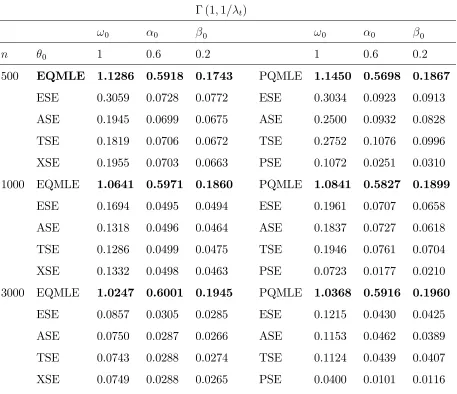
Monte Carlo experiments, not presented here for the sake of brevity, confirm the asymptotic

results of this section in finite samples.

5

Testing the multiplicative form of duration models

Instead of a standard ACD duration model (1.2), the present paper suggests a more general

POLI model with a conditional distribution that is not constrained by the MEM structure.

The variablezt=Yt/λtis independent of λt:=E(Yt| Ft−1) in model (1.2), whereas the two

variables are uncorrelated but not necessarily independent in the POLI model. In particular

the conditional variance of a POLI model is not constrained to be proportional to λ2_t. It is

thus of interest to test

H0 : zt and λt are independent, (5.1)

without specifying a particular alternative model. Based on observations Y1, . . . , Yn, the

hypothesis H0 can be tested by using the empirical distance covariance (see Sz´ekely et al.

(2007), Rizzo and Sz´ekely (2016), and the references therein)

Vn2 =

Z

where ϕ_bz,λ, ϕ_bz and ϕ_bλ are respectively empirical estimators of the characteristic functions of (zt, λt), zt and λt. As shown in Sz´ekely, Rizzo and Bakirov (2007), a relevant choice of

weighting function is w(t, s) proportional to t−2_s−2_{. Under the null and the existence of}

marginal moments,nV2

n converges in distribution. The limiting distribution depends on the

marginal laws of the two variablesztandλtin the iid case. Davis, Matsui, Mikosch and Wan

(2018) recently showed that the nice properties of the distance covariance and correlation

can also be extended to time series. In our framework, the sequence (zt, λt)t≥1 is not iid

under the null, and λt is not directly observable, but can be approximated by eλt(bθ) defined

by (4.2). We propose to approximate the distribution of _V2

n by the bootstrap distribution of

the variable V∗2

n defined in the following resampling scheme:

(i) Calculate the QMLE bθ = θn(Y1, . . . , Yn) defined by (4.3), the test statistics Vn2 =

V2

n(Y1, . . . , Yn), and the residualszbt =Yt/λet(bθ) for t=q+ 1, . . . , n. Denote by Fn the

empirical distribution of {zbt/sn, t = 1 +q, . . . , n} where sn =Pn_t=q+1bzt/(n−q) (with

this scaling factor, the expectation of the distribution Fn is equal to 1).

(ii) GenerateY∗

1, . . . , Yn∗whereYt∗ =zt∗eλ ∗

t(bθ), thez∗t’s are independent andFn-distributed,

andeλ∗_t(θ) is defined aseλt(θ) withYt−ireplaced byYt∗−i. Calculateθb ∗

=θn(Y1∗, . . . , Yn∗)

and the test statistics V∗2

n =Vn2(Y1∗, . . . , Yn∗).

(iv) Repeat step (ii) B times and calculate the corresponding test statisticsV∗2

n,1, . . . ,Vn,B∗2 .

(v) At the nominal significance level α _∈ (0,1), reject H0 if Vn2 > Vn,(B∗2 −[αB]), where

V∗2

n,(1) ≤. . .≤ Vn,(B)∗2 denote the corresponding order statistics.

The validity, i.e. the consistency under the null and the alternative, of an apparently sim-ilar resampling scheme has been proven in Francq, Jim´enez-Gamero and Meintanis (2017).

However, our framework is not the same, since the above-mentioned paper concerns

spheric-ity tests based on the empirical characteristic function. Proving the validspheric-ity of the present

algorithm does not seem trivial and will be the topic of future research.

Of course, when one wants to test a given ACD model against a particular POLI model, a

com-paring the likelihood of the two models. This will be illustrated in an empirical application

below.

5.1

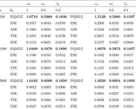
Monte Carlo experiments

We simulated two data generating processes (DGP), one which satisfies H0 and the other

which does not. The first DGP is an ACD(1,1) modelYt =λtztwhereλt=ω+αYt−1+βλt−1

with (ω, α, β) = (0.5,0.1,0.89), and thezt’s are independent with exponential distribution of

mean 1. The other DGP (denotedH1in Table1) is a POLI model of conditional distribution

Γ(bλt, b) with b = 0.01 and λt which follows the same equation as in the first DGP. We used

the resampling algorithm with B = 99 replications (in the numerical illustration of the next

subsection, we also used B = 999 and noticed that the results were similar for B = 99 and

B = 999). Table 1 displays the empirical relative frequency of rejection over N = 1000

independent replications of the two DGP’s, for the sample sizes n = 500 and n = 1000.

The exercise is computationally demanding since N _×(B + 1) _×2_×2 = 400000 models

have to be estimated and as many distance covariances have to be computed (leading to

around 3 days of computations on a personal laptop). Table 1 shows that the error of first

n= 500 n= 1000

DGP α= 1% α = 5% α= 10% α = 1% α= 5% α= 10%

H0 1.2 3.0 5.8 0.7 3.8 6.7

H1 54.0 86.0 95.2 73.8 96.5 99.2

Table 1: Percentages of rejections of the bootstrapped distance covariance test.

kind is well controlled when α = 1%, but the test is slightly conservative at levels α = 5%

and α = 10%. Indeed, over N = 1000 replications of a test with nominal level α = 1%

(respectively 5% and 10%), the empirical relative frequency of rejection should vary between

0.2% and 1.9% (respectively 3.2% and 6.9%, and 7.5% and 12.5%) with probability 0.99.

our Monte Carlo setting. Of course, for other alternative models, that omnibus test of

independence may be less powerful. For instance, when the conditional distribution of the

DGP is Γ(bλt, b) with larger b, the power is smaller. This is not surprising because the

varianceλt/bof zt∼Γ(bλt, b) is a decreasing function ofb and, since the variablezttends to

become constant when b increases, it is harder and harder to detect a relationship between

zt and any other variable.

5.2

S&P 500 transaction volume

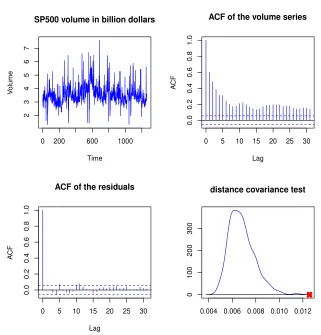
Consider the series (Yt) of the S&P 500 transaction volume from 3/10/2013 to 3/10/2018,

which corresponds to 1260 values (downloaded on Yahoo! Finance). Fitting a model (1.1)

with (p, q) = (2,1), the parameter estimates of the QMLE (4.3) are ω_b = 0.680, α_b1 = 0.498,

b

β₁ = 0.271, βb₂ = 0.040. As shown in the bottom-left panel of Figure 2, the autocorrelation function (ACF) of the residuals _bzt = Yt/eλt(bθ) no longer shows any sign of dynamics. The

distance covariance test however rejects the standard MEM-ACD model in which zt and

λt are independent. Indeed, a kernel density estimator of the bootstrapped distribution

of _V2

n under the null is displayed at the bottom-right panel of Figure 2. The value of Vn2

computed on the observations, indicated by a cross on the figure, is located at the extreme

right of the distribution, which gives strong evidence for rejecting the null. Actually, the

observed value of the distance covariance is larger than all theB = 999 bootstrap replications

used to approximate the distribution of _V2

n under the null. The estimated p-value is thus

1/1000 = 0.001. On a personal computer with a 2.80 GHz processor, the bootstrap-based

test run time was around 600 seconds.

The distance covariance test concludes that a non-multiplicative POLI model is better

than an ACD model for this particular series, but the test is not informative about the

distributionFλ. We therefore tried several specifications for the conditional distribution Fλ:

the Exponential (ACD), the Γ(a, a/λt) (G-ACD), the Γ(bλt, b) (G-POLI), and two additive

models of the form (2.3) in which ǫt is assumed to follow a Γ(a, b) distribution (G-Add) or

a Fisk distribution (F-Add) with density f(y) = ab(ay)b−1_{/(1 + (ay)}b₎2₁

SP500 volume in billion dollars

Time

V

olume

0 200 600 1000

2

3

4

5

6

7

0 5 10 15 20 25 30

0.0

0.2

0.4

0.6

0.8

1.0

Lag

A

CF

ACF of the volume series

0 5 10 15 20 25 30

0.0

0.2

0.4

0.6

0.8

1.0

Lag

A

CF

ACF of the residuals

0.004 0.006 0.008 0.010 0.012

0

100

200

300

distance covariance test

Figure 2: S&P 500 transaction volume from 3/10/2013 to 3/10/2018, ACF on the observed

series, ACF on the residuals of the POLI(2,2) model, distribution of the distance covariance

under the null hypothesis of multiplicative form, and observed distance covariance (cross

is a scale parameter and b > 0 is a shape parameter. For instance, the Fisk distribution is

used for hydrological stream flow modeling, or for the distribution of wealth in economics.

These models being fully parametric, they have been estimated by maximum-likelihood.

Table 2 shows that, according to the usual Akaike and bayesian information criteria (AIC

and BIC), the F-Add model outperforms the other models. This is certainly due to the

fact that the Fisk distribution can better take into account the fat tails of the conditional

distribution of the series (see the top-left panel of Figure 2) than the Gamma distribution.

Note that the Fisk distribution admits finite moments of order less than b only, while the

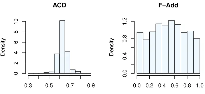
Gamma distribution admits moments of any order. Figure 3 compares the histograms of

the Probability Integral Transform (PIT) of the ACD and F-Add models, i.e. the empirical distributions ofFb_λb

t(Yt), whereλt andFλ are estimated by the MLE of the two models. Note

that if the actual conditional distribution of Yt is the continuous cdf Fλt, then Fλt(Yt) is

uniformly distributed on [0,1]. Given this graph, the ACD is clearly rejected, while there is

no visible evidence against the F-Add model. Indeed, similar PIT histograms are obtained

on simulations of the F-Add model.

ACD G-ACD G-POLI G-Add F-Add

AIC 5657.409 1871.527 1888.031 1927.031 1636.941

BIC 5677.933 1897.181 1913.685 1957.816 1667.726

Table 2: AIC and BIC of the different models for the S&P 500 transaction volume series.

5.3

Greenhouse gas concentrations

Lucaset al. (2015) studied a large network data set of greenhouse gas (GHG) concentrations collected by tracers located at different areas in California. The left panel of Figure4displays

the time series obtained by one of these tracers. The partial autocorrelogram suggests

that the simple model (1.1) with q = 1 and p = 0 could be sufficient to summarize the

ACD

Density

0.3 0.5 0.7 0.9

0

2

4

6

8

10

F−Add

Density

0.0 0.2 0.4 0.6 0.8 1.0

0.0

0.4

0.8

1.2

Figure 3: Probability integral transform (PIT) histograms for the ACD and F-Add models.

p-values of the test generally vary between 2% and 14% among the different series of GHG

concentrations. On the time series plot, one can see a concentration of observations around

zero, which precludes a continuous conditional distribution such as the Gamma law. We

thus investigated the use of zero-inflated conditional distributions. We denote by ZIE-ACD

the model of the ACD form (1.2) where zt follows a zero-inflated exponential distribution,

i.e. the model

Yt=λtzt, λt=ω+αYt−1, zt∼τ δ0(x) + (1−τ)µe−µx1x>0,

with standard notation for the mixture distribution, andµ= 1−τ in order to haveEzt = 1.

We denoted by ZIG-ACD the same model where, in the Radon-Nikodym density of zt, the

exponential distribution is replaced by the Γ(a,(1−τ)a) law. Note that the conditional

distribution of Yt is then Yt| Ft−1 ∼τ δ0+ (1−τ)Γ(a,(1−τ)a/λt). We also considered the

model

λt=ω+αYt−1, Yt| Ft−1 ∼τ δ0+ (1−τ)Γ(λtb,(1−τ)b).

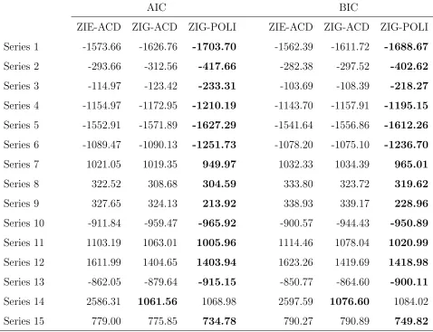
Since this model can not be written in ACD multiplicative form (1.2) (its conditional variance

been estimated by maximum-likelihood on 15 series of GHG concentrations. Table 3shows

that, according to the AIC and BIC criteria, the POLI model is almost always preferable to

the ACD models. On the series displayed in Figure4(corresponding to Series 1 of Table 3),

the maximum-likelihood estimates of the ZIG-POLI parameters areω_b = 0.0020,α_b = 0.6888,

b

τ = 0.1743 andbb= 297.0.

Time

GHG

0 50 150 250

0.00

0.02

0.04

0.06

5 10 15 20 25

0.0

0.2

0.4

0.6

0.8

Lag

P

ar

tial A

CF

Figure 4: Greenhouse gas time series concentration every 6 hours from May 10 to July 31,

2010, and empirical partial autocorrelations of the time series.

6

Conclusion

Proving the ergodicity of count time series models is a notorious tricky problem, for which

the present paper gives a simple solution. This also applies to more general positive-valued

series. In Sections 2-3, we present a unified approach to investigate stationarity and other

probabilistic properties of many, seemingly distinct, models of count and durations time

series. Section 4 shows that the approach also allows for a unified treatment in terms of

estimation of the conditional mean. The illustrations presented in Section 5 suggest that

AIC BIC

ZIE-ACD ZIG-ACD ZIG-POLI ZIE-ACD ZIG-ACD ZIG-POLI

Series 1 -1573.66 -1626.76 -1703.70 -1562.39 -1611.72 -1688.67

Series 2 -293.66 -312.56 -417.66 -282.38 -297.52 -402.62

Series 3 -114.97 -123.42 -233.31 -103.69 -108.39 -218.27

Series 4 -1154.97 -1172.95 -1210.19 -1143.70 -1157.91 -1195.15

Series 5 -1552.91 -1571.89 -1627.29 -1541.64 -1556.86 -1612.26

Series 6 -1089.47 -1090.13 -1251.73 -1078.20 -1075.10 -1236.70

Series 7 1021.05 1019.35 949.97 1032.33 1034.39 965.01

Series 8 322.52 308.68 304.59 333.80 323.72 319.62

Series 9 327.65 324.13 213.92 338.93 339.17 228.96

Series 10 -911.84 -959.47 -965.92 -900.57 -944.43 -950.89

Series 11 1103.19 1063.01 1005.96 1114.46 1078.04 1020.99

Series 12 1611.99 1404.65 1403.94 1623.26 1419.69 1418.98

Series 13 -862.05 -879.64 -915.15 -850.77 -864.60 -900.11

Series 14 2586.31 1061.56 1068.98 2597.59 1076.60 1084.02

Series 15 779.00 775.85 734.78 790.27 790.89 749.82

Table 3: Information criteria of ACD and POLI models on 15 series of GHG concentrations

This gives a motivation for relaxing the usual multiplicative form of the ACD-like models,

even if the probabilistic structure of the model is then complicated by the absence of an

explicit iid innovation sequence. Note that the positivity of the observations is not

funda-mental for some of the results. In particular, one could easily obtain sufficient stationarity

conditions without this assumption. Moreover, our results can be applied to positive-valued

transformations of a non-positive series ǫt. For example, the square of a GARCH has the

ACD form ǫ2

t = σ2tη2t where the volatility σt is independent of the iid sequence ηt. Since

the multiplicative form of the GARCH model entails strong restrictions, such as a constant

conditional kurtosis, it could be of interest to consider a POLI model on ǫ2

t. This is a topic

that we leave for future research.

A

Proofs

Proof of Lemma 2.1 Note that the result is trivial when the number of failures r1 and r2

are integers. More generally, note that the likelihood ratio

P _{N B(r2, p0) = k}

P {N B(r1, p0) = k}

=pr2−r1

0 k

Y

i=1

r2+k−i

r1+k−i

increases withk, which is known to entail the required stochastic dominance (see e.g. The-orem 1 in Lehmann (1955)).

Proof of Lemma 2.2 Assume (1.5), (2.5) and EY = (1−τ)λ ≤ EY∗ _{= (1−τ)λ}∗_{. Then}

for y _≥0 we have P(Y _≤y) =τ + (1₋τ)Fλ(y)≥τ + (1−τ)Fλ∗(y) = P(Y∗ ≤y) and the

result follows.

Proof of Theorem 3.1 Assume (1.3) with (X_t) stationary and ergodic, for which (1.1) can be considered as a particular case.

If there exists m _∈(0,_∞) such that m =EYt =Eλt for all t, then

1−

q

X

i=1

αi− p

X

j=1

βj

!

Under the positivity constraints on the parameters and exogenous variables, this equality

entails (3.2) and Eπ⊤Xt <∞.

It thus remains to show that (3.2) is sufficient for the existence of a strictly stationary

and ergodic solution to (3.1). Let (Ut) be an iid sequence of random variables uniformly

distributed in [0,1], independent of the sequence (X_t). Fort _∈Z_{, let Yt}(k) _=λ(k)_{t = 0 when}

k ≤0 and, fork >0, let

Yt(k) =F_λ−(k)

t

(Ut), λ(k)t =ω+ q

X

i=1

αiYt(k−i−i)+ p

X

j=1

β_jλ(k_t−−_jj)+π⊤Xt−1. (A.1)

Fork ≥2, we have

λ(k)_t =ψ_k(Ut−1, . . . , Ut−k+1; Xs, s < t),

where ψ_k : [0,1]k _×[0,∞)∞ _{→ [0,∞) is a measurable function. Therefore, for any k, the}

sequences λ(k)t

t and

Yt(k)

t are stationary and ergodic. Let F (k)

t−1 and Ft∗−1 be the

sigma-fields generated by nY_t(k_−i−i), i > 0;X_s, s < to and _{Us,Xs, s < t}, respectively. We have

EY_t(k) _{| Ft}(k)₋₁=EY_t(k) _{| Ft}∗₋₁=λ(k)_t , PYt(k) ≤y| F

(k) t−1

=P F−

λ(tk)

(Ut)≤y| Ft∗−1

=F_λ(k)

t (y).

We have used the well known result that F_λ−(U) has the cdf Fλ when U is uniformly

dis-tributed in [0,1]. To show the existence of a solution to (3.1), with Ft−1 replaced by Ft∗−1,

it is now sufficient to show that

λt= lim k→∞λ

(k)

t exists almost surely (a.s.) in [0,+∞). (A.2)

Taking the limit as k_{→ ∞} in both sides of the equalities in (A.1), the solution will be then

given by Yt = limk→∞Yt(k) = Fλ−t(Ut) a.s. We then note that the distribution of Yt given

F∗

t−1 is the same as that of Yt given Ft−1 since λt isFt−1-measurable.

We now show (A.2) under (3.2). We first prove that, for all k,

0≤λ(kt −1) ≤λ (k)

and

EYt(k)−Y (k−1) t

=Eλ(k)t −λ (k−1) t

∈[0,∞). (A.4)

Clearly, (A.3) and (A.4) hold true for k _≤ 0. Assume (A.3) is satisfied for k _≤k0, then

using (2.2) we have

λ(k0+1)

t =ω+

q

X

i=1

αiF− λ(k0+1−i)

t−i

(Ut−i) + p

X

j=1

βjλ

(k0+1−j)

t−j +

r

X

i=1

πixi,t−1

≥ω+

q

X

i=1

αiF− λ(k0−i)

t−i

(Ut−i) + p

X

j=1

βjλ (k0−j)

t−j +

r

X

i=1

πixi,t−1 =λ(kt 0).

Therefore the inequalities in (A.3) are shown by induction. Now note that EY_t(k) = Eλ(k)_t

exists for any fixed k, and for all positive parameters. It follows that (A.4) holds true. In

the casep=q= 1, we then have

Eλ(k)_{t −}λ_t(k−1)= (α+β)Eλ_t(k₋−₁1)₋λ(k_t−−₁2)= (α+β)k−1ω.

More generally, with obvious convention, under (3.2) we have

Eλ(k)_{t −}λ(k_t −1)=

max(p,q)_X i=1

(αi+βi)E

λ_t(k₋−_ii)₋λ(k_t−−_ii−1)_≤Kρk, _∀k_≥1,

with K > 0 and ρ _∈(0,1). This entails that the sequence nλ(k)t

o

k converges in L

1 _{and a.s.}

under (3.2). Moreover, since

λt=ψ(Ut−1, Ut−2, . . .; Xt−1,Xt−2, . . .),

where ψ : [0,1]∞_×[0,∞)∞_{→[0,∞) is a measurable function, the sequence (λ}

t) is ergodic.

Proof of Theorem 3.2 Let the notation ms = EYts when the moment exists, and b(ℓ) =

Pℓ−1

i=0aℓ(i)Eλ i

t. Then (3.3) entails mℓ=a(ℓ)Eλℓt+b(ℓ).

We first show EY2

t <∞ iff (3.4) holds with ℓ= 2. The latter condition writes

Since m2 =a(2)Eλ2t +b(2), we have

m2 = a(2)

ω2+α2m2+ 2ω(α+β)m1 + (β2+ 2αβ){m2−b(2)}+b(2)

= a(2)α2+β2+ 2αβ m2+K,

where

K =a(2)ω2+ 2ω(α+β)m1 +b(2) 1−β2 −2αβ

>0.

Therefore EY2

t < ∞ entails (A.5). To show that (A.5) is also sufficient, recall that it has

been shown in the proof of Theorem3.1 that

Yt= lim

k→∞↑Y

(k)

t .

By the monotone convergence theorem, to prove thatm2 exists it thus suffices to prove that

limk→∞m(k)2 is finite, where m (k)

s denotes EYt(k)s (which is finite for all s ≥ 0 and all k).

Letting µ(k)s =Eλ(k)st and b(k)(ℓ) =

Pℓ−1

i=0aℓ(i)Eλ(k)it we have

m(k)₂ =a(2)µ(k)₂ +b(k)(2)

= a(2)nω2+α2m₂(k−1)+ 2ω(α+β)m(k₁ −1)o

+(β2+ 2αβ)nm₂(k−1)−b(k−1)(2)o+b(k)(2) = a(2)α2+β2 + 2αβ m(k₂ −1)+K(k),

where

K(k) =a(2)nω2+ 2ω(α+β)m₁(k−1)o+b(k)(2)−b(k−1)(2) β2+ 2αβ→K

a.s. ask _{→ ∞}, since we have seen in the proof of Theorem3.1that (3.2) entails limk→∞m(k)1 =

limk→∞µ(k)1 =m1. We thus have

m(k)₂ ≤ρm(k₂ −1)+ 2K ≤2K

∞

X

i=0

ρi <∞

The proof of (3.4) is complete in the case ℓ= 2. Now consider the general case, arguing

by induction on ℓ≥3. We have

mℓ = a(ℓ)

( _ℓ X j=0 ℓ j

αjβℓ−jEY_tj₋₁λℓ_t−−j₁+Rℓ

)

+b(ℓ)

= a(ℓ)αℓmℓ+ ℓ−1

X

j=0

a(j)

ℓ j

αjβℓ−j{mℓ−b(ℓ)}+a(ℓ)R(ℓ) +b(ℓ),

where the term R(ℓ) is a linear combination of 1, Eλt, . . . , Eλℓt−1 with positive coefficients.

By induction, one can assume that R(ℓ) andb(ℓ) are finite under (3.4). It follows that (3.4)

is necessary to have mℓ finite. The converse is shown as in the case ℓ= 2.

Proof of Theorem 3.3 As in the proof of Theorem 3.1, consider an iid sequence (Ut)

of random variables uniformly distributed in [0,1], independent of the sequence (Xt), and

define Yt(k)=λ (k)

t = 0 when k ≤0 and, whenk >0,

Yt(k)=F_λ−(k)

t

(Ut), (A.6)

λ(k)_t =g(Y_t(k₋₁−1), . . . , Y_t(k_−q−q), λ_t(k₋−₁1), . . . , λ(k_t−−_pp)) +π(Xt−1).

By the argument of the proof of Theorem 3.1, to show the existence of a stationary solution

it suffices to show the almost sure convergence (A.2) of λ(k)t as k→ ∞. In view of (2.2), we

have

En_|Yt(k)−Y (k−1)

t |λ

(k) t , λ

(k−1) t

o

=λ(k)t −λ (k−1) t

.

Therefore

EYt(k)−Y (k−1) t

=Eλ(k)t −λ (k−1) t

.

It follows that, under (3.9),

Eλ(k)_{t −}λ(k_t −1)_≤

p∨q

X

i=1

(αi+βi)E

λ(k_t−−_ii)₋λ_t(k₋−_ii−1)_≤Kρk, _∀k _≥1,

for some constans K >0 and ρ∈(0,1). The proof of the existence of a stationary solution

Now assume (3.9) and Yt is valued in N. For i= 1,2, define stationary processes by

Y_t[i] =F−

λ[ti]

(Ut), λ[i]t =g(Y [i]

t−1, . . . , Y [i] t−q, λ

[i]

t−1, . . . , λ [i]

t−p) +π(Xt−1),

for t_≥1, where

Z[1]₀ = (Y₀[1], . . . , Y₁[1]_−q, λ[1]₀ , . . . , λ[1]_1−p) and

Z[2]₀ = (Y₀[2], . . . , Y₁[2]_−q, λ[2]₀ , . . . , λ[2]_1−p) are independent and follow the stationary law of

Z_t:= (Yt−1, . . . , Yt−q, λt−1, . . . , λt−p).

By the coupling arguments used to show (5.6) in Davis and Liu (2016) or (5.9) in Neumann

(2011), we have

β(h) =Esup

A∈B|

P _{(Yh, Yh+1, . . .)∈A|Z0} −P {(Yh, Yh+1, . . .)∈A}|

=Esup

A∈B

P n(Y_h[1], Y_h+1[1] , . . .)_∈A_|Z[1]₀ o₋P n(Y_h[2], Y_h+1[2] , . . .)_∈A_|Z[1]₀ o

≤

∞

X

k=0

P Y_h+k[1] 6=Y_h+k[2] ≤

∞

X

k=0

EY_h+k[1] −Y_h+k[2] ,

with obvious notation. The last inequality holds becauseY_h+k[1] ₋Y_h+k[2] is valued in N_{. Now,}

note that (2.2) implies that

E|Yt[1]−Y [2]

t |λ

[1] t , λ

[2] t

=|λ[1]t −λ [2] t |.

Therefore

E|Yt[1]−Y [2]

t |=E|λ [1]

t −λ

[2]

t | ≤

q

X

i=1

αiE|Yt[1]−i−Y [2] t−i|+

p

X

j=1

βjE|λ [1] t−j −λ

[2]

t−j| ≤Kρt,

and the conclusion follows.

Lemma A.1 Let _{Yt, t∈Z} be a strictly stationary and ergodic sequence satisfyingA1and A2. Assume that Θsatisfies the compactness assumption A6. There exist a F0-measurable

random variable K >0 and a constant ρ_∈(0,1) such that

sup

θ_∈Θ

λt(θ)−eλt(θ)

Proof of Lemma A.1 By (3.8), fort _≥q+ 1 we have

δt:=

λt(θ)−eλt(θ)

≤

p

X

j=1

β_jλt−j(θ)−eλt−j(θ)

≤β max

j=1,...,pδt−j,

where β := supθ_∈Θ

Pp

j=1βj < 1 by A2 and A6. Iterating the previous inequality, and

setting K0 = supθ_∈Θmaxj=1,...,pδq+1−j, we obtain

δq+1 ≤K0β, δq+2 ≤βmax{δq+1, K0} ≤K0β, δq+j ≤K0β, j = 1, . . . , p

δq+p+j ≤K0β2, j = 1, . . . , p, δq+kp+j ≤K0βk+1, j = 1, . . . , p.

When β = 0, the result is obvious. When β > 0, the result holds with K = K0β−q/p and

ρ=β1/p.

Lemma A.2 Let{Yt, t∈Z}be a strictly stationary and ergodic sequence satisfyingA1, A2

and A4, and assume A6. We have

Esup

θ_∈Θ

λt(θ)<∞.

Proof of Lemma A.2 Note that, by (3.8),

λt(θ)≤ct(θ) + p

X

i=1

β_jλt−j(θ), ct(θ) = g(0⊤;θ) +π(Xt−1) + q

X

i=1

αiYt−i.

Let λt(θ) = (λt(θ), . . . , λt−p+1(θ))⊤, ct(θ) = ct(θ),0⊤⊤ and B a companion-like matrix

such that the previous inequality yieldsλ_t(θ)≤c_t(θ)+Bλ_t−1(θ). Lettingλ_t = supθ_∈Θλt(θ)

and ct = supθ_∈Θct(θ) componentwise, we obtain

kλtk ≤ kctk ∞

X

i=0

sup

θ_∈Θk

B_ki <∞

because A2 and A6 entail supθ_∈Θρ(B)< 1 (see e.g. (7.27) in Francq and Zakoian, 2019).

The conclusion follows.

the inequality log (x)_≤x₋1,A3 and Lemma A.1, it follows that

sup

θ_∈Θ

Ln(θ)−Len(θ)

= 1

nsupθ_∈Θ

n X t=1 Yt 1

λt(θ) −

1

e

λt(θ)

!

+ log λt(θ)

e

λt(θ)

!! ≤ 1 n n X t=1 

Ytsupθ∈Θ

λt(θ)−eλt(θ)

λt(θ)eλt(θ)

+ supθ∈Θ

eλt(θ)−λt(θ)

e

λt(θ)

  ≤ K n n X t=1

Ytρt

ω2 +

ρt

ω

→0,a.s. asn _{→ ∞}. (A.7)

B