Munich Personal RePEc Archive
Mortgage Supply and Housing Rents
Gete, Pedro and reher, Michael
IE Business School, Harvard University
November 2017
Online at
https://mpra.ub.uni-muenchen.de/82856/
Mortgage Supply and Housing Rents
Pedro Gete
yand Michael Reher
zThis Draft: October 2017
Abstract
We show that a contraction of mortgage supply after the Great Recession has increased housing rents. Our empirical strategy exploits heterogeneity in MSAs’ exposure to regula-tory shocks experienced by lenders over the 2010-2014 period. Tighter lending standards have increased demand for rental housing and have led to higher rents, depressed home-ownership rates and an increase in rental supply. Absent the credit supply contraction, annual rent growth would have been 2.1 percentage points lower over 2010-2014 in MSAs where lending standards rose from their 2008 levels.
Keywords: Credit Supply, Homeownership, Mortgage Markets, Regulation, Rents.
JEL Classi…cation: G18, G21, G28, R21, R38
We thank Sumit Agarwal, Jim Albrecht, Brent Ambrose, Elliot Anenberg, Neil Bhutta, John Campbell, Mark Carey, Brian Chen, Stijn Claessens, Behzad Diba, Gabriel Chodorow-Reich, Ricardo Correa, Edward DeMarco, Jihad Dragher, Martin Evans, Ammar Farooq, Jesus Fernandez-Villaverde, Benjamin Friedman, Carlos Garriga, Lei Ge, Ed Glaeser, Laurie Goodman, Sam Hanson, John Halti-wanger, Anil Jain, John Krainer, Tim Landvoight, Steven Laufer, John Leahy, Deborah Lucas, David Marques-Ibanez, Atif Mian, Raven Molloy, Whitney Newey, Jonathan Parker, Franco Peracchi, Daniel Ringo, John Rogers, Kevin Roshak, Antoinette Schoar, Kamila Sommer, Viktors Stebunovs, Jeremy Stein, Philip Strahan, Susan Vroman, Nancy Wallace, Paul Willen, anonymous referees and seminar participants at the 2016 AREUEA Conference, 2016 MIT Golub Center Conference, 2017 ASSA, Board of Governors of the Federal Reserve, Georgetown, and Harvard for comments. Pedro Gete gratefully acknowledges the …nancial support of the Spanish Ministry of Economy and Competitiveness Grant No. ECO2014-53022.
1
Introduction
This paper shows that a contraction of mortgage credit supply has been a signi…cant driver of housing rents and homeownership since the 2008 crisis. Following the crisis, homeownership rates collapsed to historic lows while housing rents increased rapidly in many U.S. cities. For example, real rents grew by more than 23% in the top 10% of fastest growing MSAs over the 2011-2014 period. During these years, the median U.S. rent-to-income ratio increased by more than in the previous 35 years. The large number of cost-burdened renters has prompted policy debates about what to do (Fernald et al. 2015).
The mechanism that we test was originally proposed by Linneman and Wachter (1989) and is formalized by Gete and Reher (2016).1 It begins with a shock that contracts mortgage supply
for some lenders such as, for example, greater regulatory costs because of stress-testing. Then, frictions to substitute across lenders lead to more di¢cult access to credit. Since downward house price rigidities prevent most households from buying without credit, households denied credit move from the market for homeownership to the rental market. An increase in the demand for rental housing, together with an imperfect short-run elasticity of supply, drives up housing rents and reduces homeownership rates. Lower price-to-rent ratios encourage investors to buy owner occupied units and convert them to rentals.
Our identi…cation strategy exploits heterogeneity across MSAs in exposure to lenders which su¤ered regulatory shocks following the Dodd-Frank Act, approved in 2010. We ask whether MSAs with greater exposure to these credit supply shocks experienced higher rent growth. The challenge for our identi…cation is to isolate credit supply shocks from other shocks that drive both housing rents and mortgage denial rates, our measure of mortgage supply. For example, an OLS regression of mortgage denial rates on housing rents would be biased if a negative shock to local activity results in credit stringency, while also dampening rent growth through reduced amenities.
We use an instrumental variables approach to surmount the previous challenge. Our pre-ferred instrument is the 2008 mortgage application share of lenders which underwent a capital stress test between 2011-2015. Since the bank distribution that we use was determined prior to Dodd-Frank, there is no risk of reverse causality. Calem, Correa, and Lee (2016) document that stress tests are associated with tightened standards in mortgage markets. We also explore as a second instrument MSA exposure to the Big-4 banks using a pre-determined measure of bank distribution across markets, the branch deposit share in 2008 from the FDIC’s Summary
1Ambrose and Diop (2014) and Acolin et al. (2016) provide empirical support using di¤erent periods and
of Deposits.2 Stein (2014) discusses how Dodd-Frank has exposed the Big-4 banks to
height-ened oversight and higher liquidity and capital requirements. Jayaratne and Strahan (1996) document the importance of bank branches in facilitating access to credit, and since their sem-inal work a number of papers have exploited bank branch distributions to create credit supply instruments (e.g. Nguyen 2016). Finally, we explore as a third instrument the share of top 20 lenders active in 2007. D’Acunto and Rossi (2017) use this instrument to study a regressive redistribution of mortgage credit between 2011 and 2014 stemming from post-crisis …nancial regulation.
We rigorously assess the validity of the instruments. First, we control thoroughly for an array of local activity shocks, pre-crisis trends and borrower and lender characteristics, making it unlikely that the error term re‡ects common movers of both mortgage supply and rents. Second, we provide extensive evidence that in the pre-Dodd-Frank period the instruments do not correlate with either higher rents or with other factors that cause rent growth. For example, before 2010 there are parallel patterns between MSAs with the highest and lowest exposure to the Big-4 and stress tested lenders. Third, placebo tests con…rm that the instruments only capture post-crisis credit supply shocks. Fourth, overidenti…cation tests are supportive of the instruments’ validity. This suggests that we are identifying similar credit supply e¤ects with di¤erent underlying variation.
All the speci…cations point in the same direction: tighter credit caused higher housing rents over 2010-2014. Our baseline speci…cation suggests that a 1 percentage point increase in denial rates increased rent growth by 1.3 percentage points. To put this estimate into perspective it is useful to look how denial rates changed over 2010-2014. Over this period average denial rates fell by 1.6 percentage points relative to their 2008 levels. However, denial rates actually rose in 31% of MSAs. Our estimates indicate that rents would have grown at least 2.1 percentage points less in these MSAs if their denial dates had moved with the national average. This e¤ect is equal to 70% of a cross-sectional standard deviation in 2010-2014 rent growth. Thus, elevated post-crisis credit stringency explains a meaningful amount of cross-MSA variation in recent rent behavior.
Consistent with the theory, the credit shock captured by our instruments lowered price-to-rent ratios and had a non-positive e¤ect on housing prices. The e¤ect is more negative for starter homes, which are more likely priced by constrained buyers. In MSAs more exposed to the credit supply shock, the correlation between prices and rents is negative, and especially so where more households face binding borrowing constraints, proxied by a higher minority share. The credit shock encouraged the conversion of owner occupied units to rentals and lowered the
homeownership rate.
The previous results are not only supportive of our theory, but they also provide more evidence to rule out the possibility that unobserved housing demand shocks violate the exclusion restriction. If that were the case and the MSAs more exposed to our credit instruments also experienced positive demand shocks, then we might observe not only a positive and signi…cant relationship between instrumented denials and rents but also between instrumented denials and prices. This is because demand shocks can generate comovement between prices and rents as
shown in Gete and Reher (2016) and Gete and Zecchetto (2017) among others.3 However,
we …nd no evidence to support this concern. House price dynamics strongly suggest that our results are due to a credit supply contraction operating through a tenure choice channel.
The instruments’ inability to explain housing rents in a placebo exercise suggests that they are valid post-crisis credit supply shocks, not that the theory is invalid in the pre-crisis period. To investigate whether credit a¤ects rents in other periods, we use the Loutskina and Strahan (2015) instrument which the literature has accepted as a valid credit supply shock. Interestingly, there is a positive and statistically signi…cant e¤ect of credit supply on rents over the pre-crisis period.4 We interpret this result, together with the placebo exercise, as further evidence of the
instruments’ validity.
As a complement to the core cross-sectional analysis, we also employ a panel identi…cation strategy that exploits within-MSA variation following various techniques in the literature. The results are qualitatively and quantitatively similar to the baseline cross-sectional study. The placebo tests are reassuring because post-crisis shocks do not explain pre-crisis rent growth. Moreover, the panel analysis shows that the divergence in lending standards between Big-4 and non-Big-4 banks, and between stress-tested and non-stress-tested lenders, is a post-2010 phenomenon.
Thus, collectively, the paper uses a broad array of empirical methodologies which suggest the same result: a contraction of mortgage supply after the Great Recession caused higher housing rents. This result does not rule out alternative explanations for rent growth, but instead highlights the importance of the credit contraction theory after rigorously accounting for these other explanations.
In terms of contribution to the literature, to the best of our knowledge this is the …rst paper
3It is also possible for demand shocks to generate no comovement if households are constrained, but we check
that this does not drive our results by extensively controlling for local business cycles. We thank an anonymous referee for pointing out this alternative possibility.
4The magnitude is much smaller than we found over the post-crisis period, likely because variation in lending
to study the role of credit supply in the dynamics of post-crisis housing rents.5 The existing
literature on housing rents has thus far focused on other, non-credit drivers like population ‡ows (Saiz 2007), shrinking leisure of high-income households (Edlund, Machado and Sviatchi 2015), income growth (Hornbeck and Moretti 2015, or Muehlenbachs, Spiller and Timmins, 2015) or households’ expected duration of stay in a house (Halket and Pignatti 2015). Mezza et al. (2016) show that student debt has a¤ected the demand for homeownership.
In terms of empirical strategy, our paper complements Chen, Hanson and Stein (2017), D’Acunto and Rossi (2017) and Goodman (2017). Chen, Hanson and Stein (2017) show that a credit supply shock experienced by the Big-4 banks led to a contraction of small business credit and caused higher unemployment. Their identi…cation strategy is similar to our use of a Big-4 instrument, and we control carefully for the factors they highlight, like establishment creation, to alleviate concerns that local economic conditions are driving the results. D’Acunto and Rossi (2017) document that U.S. …nancial institutions have reduced mortgage lending for medium-sized loans and increased lending for large loans since the crisis. They conclude that this resulted from a supply-side change, namely the increase in the costs of originating mortgages imposed by Dodd-Frank. We show that our results hold if we use their instrumental variable to capture the e¤ect of a contraction of credit on housing rents. Goodman (2017) documents that mortgage credit has become very tight in the aftermath of the …nancial crisis and discusses potential regulatory causes of this contraction.
There is an ongoing debate on what caused the crisis and what the appropriate policy re-sponses are. Mian and Su… (2009) provide evidence pointing to excessive credit supply towards low-income households as the cause of the crisis. Adelino, Schoar and Severino (2016) or Foote, Loewenstein and Willen (2016) argue that loans to low-income households were not the dom-inant driver of pre-crisis credit ‡ows, and thus policies should not necessarily aim to restrict credit accessibility for these borrowers. Our results show that policy reforms have especially re-duced the ‡ow of credit towards households on the margin of homeownership and caused higher housing rents. However, these increases should be transitory since we also show an increase in rental supply. From a welfare perspective, it is not clear whether the decrease in homeown-ership is good or bad. For example, we document that pre-…nancial crisis lending standards were exceptionally low. The standards have tightened since the crisis, perhaps overshooting the pre-boom conditions.
5There is a large literature that analyzes whether easy access to credit caused the pre-crisis increase in house
The rest of the paper is organized as follows: Section 2 discusses the underlying theory; Section 3 has our baseline analysis; Section 4 provides multiple tests to assess the exclusion restriction; Section 5 studies house prices, homeownership and rental supply; and Section 6 concludes. The appendix explains our data sources, and the online appendix contains additional results and details on the panel methodology.
2
Motivation and Theory
In this section we describe the theory that we want to test. As Figure 1 shows, following the recent …nancial crisis, housing rents have increased steeply in many MSAs. The rent-to-income ratio for the median MSA has risen by more following the Great Recession than it did over the previous 25 years combined. At the same time, the U.S. homeownership rate has collapsed to historic lows.6
These previous facts suggest an important role for the extensive margin of rental demand, which is analyzed theoretically in Gete and Reher (2016) and Gete and Zecchetto (2017). Here we brie‡y sketch the main mechanisms that we will test later in the paper. Households can decide to buy or to rent. Thus there are two housing stocks: one for owner occupied units and another for rentals. The rental stock is owned by the wealthy households (e.g. landlords or investors). Since houses are large and indivisible goods, their purchase requires mortgage credit for all except for the wealthiest households. Households decide their tenure choice by comparing the utility from rental versus owner occupied housing, the price-to-rent ratio, and the cost and availability of mortgage credit. Mortgage lenders set their lending standards such that lenders’ expected revenue, after taking into the account the possibility of default, equals their cost of funds.
Higher costs for the lender, for example, because of higher capital requirements or the costs associated with stress-testing, shift the credit supply curve inward. Consequently, more households are denied credit at pre-shock conditions. Tighter lending standards make some households unable to borrow at the conditions they want and, given downward rigidities in house prices, they decide to rent. Higher demand for rental housing, together with an inelastic supply and imperfect convertibility between rental and owner-occupied units, lead to higher rents, lower homeownership and lower house prices. As the price-to-rent ratio falls, there are investors who buy owner occupied properties and place them for rent. That is, the tenure conversion rate increases. This "buy to let" behavior then induces a positive correlation between
rents and prices. Moreover, new construction further increases the supply of rental housing.
We check that the data support the predictions of the previous theory. Sections 3 and 4 study housing rents, and Section 5 analyzes the remaining implications.
3
Mortgage Supply and Rent Growth
This section estimates the e¤ect of credit supply on housing rents. The next section discusses the validity of the instrumental variables that we use to identify credit supply.
3.1
Database
We measure credit supply using mortgage denial rates to avoid capturing any e¤ect from borrowers’ reaction to a loan o¤er.7 Our data come from the Home Mortgage Disclosure Act
(HMDA) which we merge with rent data from the Zillow Rent Index (ZRI) and other controls at the MSA level.8 The units of the ZRI are nominal dollars per month for the median property in
the MSA. We study MSAs as the unit of analysis, as they are arguably the smallest geographical unit in which households cannot borrow in one location to purchase a house in another one.
To focus on households contemplating whether to rent or own, we only study applications for the purchase of owner-occupied, 1-to-4 family dwellings, which include single-family houses and also individual units within multi-unit buildings, such as condominiums. Table 1 contains summary statistics of the key variables in our analysis. A detailed description of all the data sources and cleaning procedures is in the Data Appendix.
3.2
Speci…cation
We focus on di¤erences at the MSA level over the 2010-2014 period, since 2010 was the year when Dodd-Frank was approved. Our baseline speci…cation is
Avg Rent Growthm;10-14= Avg Denial Ratem;10-14+ Xm+um; (1)
7Denial rates are strongly correlated with proxies for lending standards. For example, Vojtech, Kay and
Driscoll (2016) …nd that denial rates are closely linked to measures of tightening standards from the Senior Loan O¢cer Opinion Survey (SLOOS).
8Zillow computes this index by imputing a rent for each property in an MSA based on recent rental
where m indexes MSAs, Avg Denial Ratem;10-14 denotes the average denial rate over
2010-2014 and Avg Rent Growthm;10-14 denotes average annual rent growth over 2010-2014.9 The
controls inXm account for both pre-crisis dynamics as well as level e¤ects, including: the
2000-2008 average annual change in log median income, log median rent, log median house price, log population, log median inhabitant age, and unemployment rate; and the 2009 level of log median income, log median rent, log population, log median inhabitant age, and unemployment rate. We also include state …xed e¤ects in all speci…cations.
If we estimate (1) using OLS, we would obtain biased estimates. This is because local
shocks can drive both rent dynamics and mortgage supply. For example, a positive shock to an MSA’s economic activity would increase amenities and thus rent growth, while raising households’ income, thus reducing mortgage denials. As a result, the OLS estimate would be biased downward. Another possibility is that households rent due to a lack of employment opportunities, so that OLS would produce upward bias.10 Regardless of the direction of the
bias, we aim to overcome it by proposing two credit supply instruments for which there is extensive evidence that the exclusion restriction is satis…ed.
3.3
The Instrumental Variables
We study two instrumental variables that capture an MSA’s exposure to lenders facing regulatory risk over the 2010-2014 period, where the exposure is measured with pre-determined variables unrelated to the factors the literature has identi…ed as drivers of housing rents. After describing the instruments, we provide evidence that they are uncorrelated with local shocks but indeed correlated with denial rates.
Our preferred instrument is MSA exposure to lenders subject to a Comprehensive Capital Analysis and Review (CCAR) stress test between 2011 and 2015. These tests are meant to ensure that the largest bank holding companies have enough capital to weather a …nancial crisis, but as a side-e¤ect they have encouraged those institutions to tighten their standards in mortgage markets (Calem, Correa, and Lee 2016). We measure an MSA’s exposure to these lenders using their pre-shock, 2008 mortgage application share. The results are similar if we instead weight by deposit share. We prefer the 2008 application share because several
CCAR-9We use average variables because with persistent but non-permanent credit supply shocks it is inappropriate
to estimate (1) using growth in denials as the independent variable. This is because, as we show in Figure A2 of the online appendix, our credit supply shocks are strongest in the beginning of the 2010-2014 window. Thus they are positively correlated with average denial rates over this period but, because of mean reversion, negatively correlated with growth in denials.
tested lenders like Ally conduct their mortgage business through non-depository subsidiaries.
We also employ a second instrument which builds on how the Big-4 banks are the only major mortgage lenders o¢cially designated as systemically-important …nancial institutions (SIFIs) over 2010-2014. Importantly for the purposes of identi…cation, the SIFI designation is not based on an institution’s behavior in mortgage markets. Stein (2014) describes how the Dodd-Frank Act subjected the Big-4 banks to heightened oversight and higher liquidity and capital requirements. As we show formally in the panel analysis of Section 4, these lenders have tightened credit signi…cantly relative to other lenders since 2010, and thus di¤erential exposure to these lenders constitutes a credit supply shock. To measure exposure to the Big-4, we compute the Big-4’s branch deposit share in an MSA in 2008, using the FDIC’s Summary of Deposits. The results are the same if we instead weight by the number of branches.
Our key identi…cation assumption is that, once we control for a broad array of factors and …xed e¤ects, exposure to the Big-4 banks and stress tested lenders is uncorrelated with other drivers of rent growth over 2010-2014. We devote Section 4 to discuss multiple tests that all suggest that the instruments satisfy this exogeneity assumption.
The second assumption is that both instruments are relevant, that is, correlated with denial rates. Figure 2 provides visual support and shows strong correlation between the instruments and average denial rates over 2010-2014. Moreover, in all our results we test for and reject underidenti…cation.
3.4
Baseline Results
Table 2 contains the estimates of the baseline speci…cation (1). In the …rst column we estimate (1) using OLS, …nding a positive but statistically insigni…cant point estimate. However, after accounting for the endogeneity of denial rates in the second column of the table, the instrumental variables estimate suggests an economically and statistically signi…cant impact of mortgage supply on rent growth over 2010-2014. A 1 percentage point increase in denial rates increased rent growth by 1.3 percentage points.
stringency explains a meaningful amount of cross-MSA variation in recent rent behavior.
4
Validity of the Instruments
This section is devoted to assessing the instruments’ validity and in particular the exclusion restriction. To address the exclusion restriction we perform the following exercises: 1) parallel trends analysis; 2) inspection of correlation with standard drivers of housing rents; 3) extensive local business cycle controls; 4) overidenti…cation tests and sensitivity to alternative instru-ments; 5) placebo tests; 6) robustness of the results using county-level data and geographic subsamples. Moreover, we check that the results are robust to functional form using a panel approach popular in the literature since Favara and Imbs (2015).
4.1
Parallel Trends
Figure 3 plots annual rent growth for MSAs ranking in the top and bottom 25% of exposure to each instrument. The year 2010 is the critical year when the Financial Stability Oversight Council was created and CCAR stress tests were announced as part of Dodd-Frank. For both instruments, we notice a substantial divergence in post-2010 rent growth between MSAs with high versus low exposure. However, prior to the shock, there are parallel dynamics between treated and control groups. That is, the instruments appear to only be driving rents in the post-crisis period.
4.2
Correlation with Standard Drivers of Housing Rents
As an alternative test, in Table 3 we regress each of our instruments on a variety of pre-crisis trends and MSA controls. To better gauge the magnitude of these partial correlations, the table normalizes all variables to have a variance of one. This allows us to assess both the magnitude and statistical signi…cance of any correlations.11
While it is impossible to directly test the exclusion restriction, Table 3 suggests that the instruments satisfy it as there is no relevant correlation between common drivers of rent growth
11In Table 3 we use homeownership data from the decennial census because it covers a larger cross-section of
and exposure to either stress tested lenders or the Big-4 banks. Moreover, as Mian, Su…, and Rao (2013) point out, …xed di¤erences such as in the level of house prices or population will be di¤erenced out in our baseline speci…cation. Most importantly, all our regressions include an expansive set of controls.
4.3
Business Cycle E¤ects
To rule out the possibility that local business cycles drive the results, or that the results are a side e¤ect of the small business loan contractions studied by Chen, Hanson, and Stein (2017), Table 4 re-estimates our baseline instrumental variables speci…cation from Table 2 after controlling for a wide range of local business cycle variables.
In particular, Table 4 controls for …ve measures of contemporaneous economic activity in an MSA: average annual growth in unemployment, labor force participation, log number of estab-lishments, log real GDP per capita, and log median hourly wage from 2010-2014. Moreover, we control for a manufacturing labor demand shock following Adelino, Ma, and Robinson (2017).12
Regardless of which measure we use, Table 4 shows that the point estimate for the e¤ect of mortgage denials on rent growth is consistently between 1.1 and 1.3 and statistically signi…cant. Moreover, the various business cycle measures all enter with the correct sign. This suggests that regional business cycles and mortgage supply are both important for rent growth, but they operate independently.
4.4
Overidenti…cation Tests and Alternative Instruments
We now exploit overidenti…cation to assess the validity of the instrument set. First, the highly insigni…cant J-statistic in Table 2 shows that we cannot reject the null hypothesis of the instruments’ exogeneity. As an additional test, Table 5 checks the robustness of our results when using the D’Acunto and Rossi (2017) instrument: the 2007 origination share of the top 20 mortgage lenders that year.
The …rst column of Table 5 shows that the estimated e¤ect of denial rates is 1.3 when using the top 20 instrument instead of Big-4 share. This result is almost the same as in Table 2, and it is statistically signi…cant. Moreover, the overidenti…cation test continues to support the validity of all the instruments.
12In our setting this shock is the 2008 employment share of each 4-digit manufacturing industry in an MSA
To second and third columns of Table 5 use as alternative instruments the 2008 mortgage application share of lenders ranked between 20 and 50 and between 50 and 150 that year, respectively. These groupings are chosen to capture the spectrum of mid-tier lenders. In neither column do we …nd a statistically signi…cant e¤ect of denials on rent growth. This suggests that our results are not driven by local economic conditions since those factors would a¤ect all lenders and thus be re‡ected in these columns.
4.5
Placebo Test
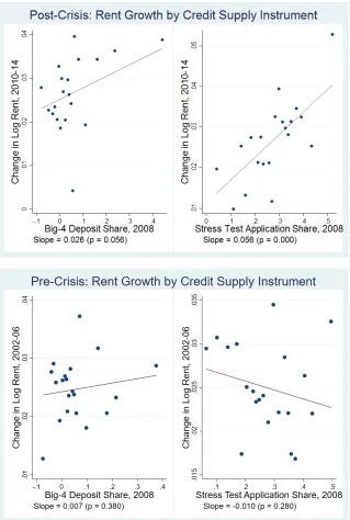
In Figure 4 we visually inspect the impact of the instruments on annualized rent growth and average denial rates over 2010-2014. The scatterplot controls for the same variables as regression (1). It is binned so that each point represents around 12 MSAs. The top panel of the …gure demonstrates strong positive correlation between each instrument and rent growth over 2010-2014. This role is absent in the pre-2008 placebo version of this …gure that is in the bottom panel of Figure 4. This evidence suggests that the instruments are not contaminated by pre-crisis rent growth.
To rigorously assess the intuition from Figure 4, we conduct various placebo tests over the 2002-2006, 2001-2005, and 2000-2004 periods. We ask if, when using a speci…cation analogous to (1), the credit supply shocks can explain rent growth over any of these periods. We should expect no e¤ect of our instruments on pre-crisis rent growth because the instruments correspond to speci…c shocks to U.S. mortgage lenders over 2010-2014, unrelated to other drivers of housing rents. The placebo point estimates in Table 6 are insigni…cant across periods, and with the opposite sign relative to Table 3. This result suggests that the instruments are truly capturing post-crisis credit supply shocks.
4.6
Sample Sensitivity
4.7
Panel Analysis
In this subsection we check the robustness of the results using a panel analysis that exploits within-MSA variation. Following Favara and Imbs (2015) we estimate
log(Rentm;t) = Deniedm;t+ Xm;t+ m+ t+um;t; (2)
where Deniedm;t denotes the one year change in the denial rate in MSAmbetween yeart 1
and yeart. This methodology allows us to hold …xed unobserved drivers of average rent growth over the sample period. However, it necessitates the use of credit supply instruments which vary over time. We study several candidates: …rst, a well-known instrument, the conforming loan limit instrument popularized by Loutskina and Strahan (2015), which we use to study the pre-crisis period and then modify for use after the 2008 Economic Stimulus Act; then the panel versions of the cross-sectional instruments studied in Section 3 that we create using the methodology of Khwaja and Mian (2008); and …nally an instrument that is agnostic about which lenders are subject to shocks, in the spirit of Greenstone, Mas and Nguyen (2015).13
4.7.1 Credit and Rents After the Crisis: Panel Analysis
The Khwaja and Mian (2008) methodology extracts a measure of lenders’ propensity to deny a loan that is purged of borrower, MSA, and time e¤ects. Figures A4 and A5 in the online appendix plot these denial propensities based on partitioning lenders according to Big-4 versus non Big-4 lenders, and according to stress tested lenders versus non-tested lenders.
Figure A4 shows that the Big-4 banks tightened standards after the implementation of Dodd-Frank and other major regulations in 2011.14 Interestingly, we see little signi…cant di¤erence
between Big-4 and non Big-4 lenders over the 2000-2003 period. This result is consistent with Big-4 exposure representing a post-crisis credit supply shock.15
Figure A5 shows that denial propensities by stress tested lenders remained elevated through-out the post-crisis period, and they increased in 2012. This was the …rst year that CCAR results were made public. The placebo pre-crisis period in the bottom panel shows little signi…cant di¤erence between the two groups of lenders, nor is there signi…cant di¤erence relative to the
13The construction of these instruments is described in the online appendix.
14Figure A6 shows how this e¤ect was especially pronounced among FHA loans, which are intended for
lower-income borrowers.
15In the top panel, the reference lender-year is non Big-4 lenders in 2007, and in the bottom panel the reference
reference lender-year (non-tested lenders in 2004). This is again consistent with exposure to stress-testing representing an exclusively post-crisis shock.
Table A4 contains the baseline panel results. As in the cross-sectional analysis, we begin by estimating (2) using OLS. The result suggests no signi…cant impact of credit supply of rents. However, after correcting for endogeneity with the instruments, the second column obtains a point estimate of 2.1 for the parameter of interest, which is very close to the estimate from Section 3.4. Furthermore, we reject the null hypothesis that the model is underidenti…ed, and the highly insigni…cant J-statistic provides evidence of the instruments’ exogeneity.
Table A5 performs a panel placebo test.16 The Big-4 and stress test panel instruments
should fail to explain rents during the pre-crisis placebo window. Indeed Table A5 shows no economic or statistical signi…cance. Moreover, the point estimates are negative. This …nding suggests that the instruments capture credit supply shocks unique to the post-crisis period.
4.7.2 Credit and Rents Before the Crisis: the Conforming Loan Limit Instrument
None of the instrumental variables speci…cations that we studied before was able to explain housing rents in the pre-crisis period. We believe this suggests that the instruments are valid post-crisis credit supply shocks, not that the theory is invalid in the pre-crisis period. To investigate whether credit a¤ects rents in other periods, we use the Loutskina and Strahan (2015) instrument which the literature has accepted as a valid credit supply shock. Thus, we use the triple product of: (a) the fraction of applications from MSAm in yeart 1within 5% of the conforming loan limit in year t; (b) MSA m’s elasticity of housing supply as estimated by Saiz (2010); and (c) the change in the log conforming loan limit between yeart 1and year
t.
The results in online appendix Table A6 suggest a positive and statistically signi…cant e¤ect of credit supply on rents in the pre-crisis period. However, the magnitude is much smaller than we found over the post-crisis period, as it suggests a 1 percentage point increase in denials led to a 0.07 percentage point increase in rent growth.17 Most importantly for this paper, Table
A6 suggests that credit supply can a¤ect rents in any period. We interpret this result, together with the result that none of the instruments used in Section 3 can explain housing rents in the pre-crisis period, as further evidence that those instruments just capture post-crisis credit
16The online appendix provides other validity tests, including tests of instrument sensitivity.
17One explanation is that there was little variation in credit supply over the pre-crisis period, as suggested by
supply shocks.
5
Channels
The previous two sections robustly documented that tight credit supply has increased rent growth. To assess whether tenure choice is indeed the relevant mechanism, we now test …ve additional implications of the theory discussed in Section 2. First, mortgage denials should lead to lower price-to-rent ratios and have a non-positive e¤ect on house price growth.18 Second, as
rents rise, "buy to let" investors convert owner occupied units to rentals. Third, the homeown-ership rate must fall due to the combined e¤ects of tight credit and expanding rental supply. Fourth, rental demand stimulates construction of multifamily units. Fifth, the credit-to-rent channel should be stronger where it is more di¢cult to substitute across lenders, for example because of di¤erent regulatory requirements across mortgage markets.
5.1
House Prices
Our theory implies that, at least in the short run, price-to-rent ratios should fall and there should be zero or possibly a negative e¤ect on house prices. To test this hypothesis, the …rst column of Table 7 re-estimates (1) replacing the outcome variable with the average growth in the price-to-rent ratio over 2010-2014. The point estimate is negative and statistically signi…cant, consistent with the theory.
In columns two and three of Table 7, we study house price growth directly. The second column restricts attention to starter homes, since these houses are more likely to be priced by households denied mortgage credit and are thus more likely to have a negative price re-sponse.19 In the third column we study all homes. In neither column do we …nd a signi…cant
e¤ect of mortgage denials on house prices, and the point estimate for starter homes is indeed substantially more negative in magnitude than the estimate obtained using all homes.
Figure 5 provides complementary visual evidence of the relationship between rent and price growth for starter homes. For MSAs with high exposure to the credit supply instruments, de…ned as an above-median value for both instruments, there is a negative relationship between rent and price growth. By contrast, the relationship between rents and prices is positive for
18We are very grateful to the editor for this suggestion.
19The price of starter homes is measured using Zillow’s Bottom Tier Index, which tracks the median home
MSAs with low exposure. Consistent with Table 7, the credit supply shock led to a substitution between rental and owner occupied properties for households denied a mortgage.
Online appendix Table A8 corroborates the previous …nding by estimating an OLS speci…-cation where the key independent variables are the 2008 mortgage applispeci…-cation share of stress tested lenders, our preferred credit supply instrument, and its interaction with an indicator of whether the MSA had an above-median share of mortgage applications from blacks or Hispanics in 2009.20 The outcome variable is the average change in house prices over 2010-2014. The idea
is that minority borrowers are more likely on the margin of homeownership. Thus markets with a high minority share may even see a negative relationship between the credit supply shock and house prices as these borrowers substitute between rental and owner occupied properties. This is indeed what we …nd, with a negative and signi…cant point estimate on the interaction term.
These results are not only supportive of our theory, but they also contribute to rule out the possibility that unobserved housing demand shocks violate the exclusion restriction. If that were the case and the MSAs more exposed to our credit instruments also had positive demand shocks, then we should observe not only a positive and signi…cant e¤ect between instrumented denials and rents but also between instrumented denials and prices. This is because demand shocks generate comovement between prices and rents as shown in Gete and Reher (2016) and Gete and Zecchetto (2017) among others. Table 7 shows no evidence supporting that argument. Thus, the dynamics of prices reported in Table 7 strongly suggest that our results in Table 2 are due to a credit supply contraction operating through a tenure choice channel.
5.2
Tenure Conversion
The decoupling of rent and price growth from Table 7 suggests a pro…table opportunity for "buy to let" investors. One would therefore expect to see increased conversion of owner occupied properties to rental units. Using data from the American Housing Survey (AHS), which tracks the same housing unit over time, we compute the fraction of rental units in an
20Following Angrist and Pischke (2009) we avoid estimating instrumental variable models with interactions
and instead Table A8 estimates:
Avg House Price Growthm;10-14= 1 Testedm;08+ 2 Testedm;08 High Minoritym;08+ Xm+um; (3)
where Avg House Price Growthm;10-14is the average annual change in the log of the Zillow Home Value Index
over 2010-2014, Testedm;08 is the 2008 mortgage application share of lenders which underwent a stress test
between 2011-2015, and High Minoritym;08indicates whether the MSA had an above-median share of mortgage
MSA which were owner occupied in the previous period.21 Then, we test the "buy to let"
channel by re-estimating (1) replacing the outcome variable with the MSA’s tenure conversion rate over 2011-2013.22
Table 8 contains the results of this exercise. In the …rst column, we …nd a positive and statistically signi…cant e¤ect of mortgage denial rates on tenure conversion. This is consistent with investors responding to a credit-induced demand for rentals by purchasing owner occupied units and subsequently renting them out.
In the second column of Table 8, we look for a longer-term e¤ect by replacing the outcome variable with the tenure conversion rate over 2003-2013. The highly insigni…cant point estimate suggests that the post-crisis credit supply shock did not raise tenure conversion rates relative to pre-crisis levels. This …nding relates to the welfare question of whether the shock led to abnormally tight standards and high rental demand, or whether it helped correct abnormally loose standards and low rental demand during the boom period. For example, online appen-dix Figure A3 shows how the spike in mortgage denials in 2010 did not raise the denial rate substantially above pre-boom levels. We leave welfare questions for future research.
5.3
Homeownership
A key implication of our theory is that the homeownership rate falls as households cannot obtain mortgage credit and the stock of rental units grows. Using data on MSA-level homeown-ership rates from the Housing Vacancy Survey, we replace the outcome in (1) with an MSA’s average growth in homeownership from 2010-2014. The results in Table 9 indicate that a one percentage point increase in mortgage denials over 2010-2014 reduced homeownership growth by 0.7 percentage points. This e¤ect is signi…cant with a p-value of 0.05 despite the relatively small sample size. This again provides evidence that tight mortgage supply raised rents through households’ tenure choice.
5.4
Multifamily Construction
We now ask whether the supply response documented in Section 5.2 was also accompanied by construction of new multifamily units. Speci…cally, we look at the growth in permits for the
21We exclude vacant units in our analysis.
construction of multifamily units.23 We replace the outcome variable in (1) with the average
growth in log multifamily permits over 2011-2014, where we o¤set the outcome window by one year to account for a lag in the supply-side response because of lengthy permitting procedures (Gyourko, Saiz, and Summers 2008). Table A9 in the online appendix suggests that the recent rent growth we have documented may dissipate as rental supply expands.
5.5
Lending Frictions
Implicit in our previous analysis is the notion that borrowers cannot easily substitute between lenders of di¤erent stringency. To measure the ease of substitutability, we utilize geographic variation in the regulation of mortgage brokers. According to Backley et al. (2006), states with additional licensing requirements for mortgage brokers have less competition, and likely stickier broker-lender relationships. That is, brokers may keep referring customers to the same lenders even if their standards are higher.24
We test the strength of these frictions with an OLS regression in which the key independent variables are the stress test credit supply instrument and its interaction with an indicator of whether the MSA is in a state requiring such licensing.25 Online appendix Table A10 has the
results. Notably, the estimated interaction term is positive and signi…cant. This suggests a role for lending frictions in strengthening the credit-to-rent mechanism on which our theory is based.
6
Conclusions
In this paper, we showed that tighter mortgage credit can explain a signi…cant component of rent growth following the 2008 …nancial crisis. Our empirical strategy used variation among MSAs in exposure to lenders more subject to regulatory costs and stress testing. We controlled for an array of local shocks and performed a battery of tests to check the validity of all
instru-23We de…ne multifamily units as the sum of 2 unit shelters, 3-4 unit shelters, and 5+ structure shelters. We
cannot disentangle whether the new buildings will contain rental or owner occupied units.
2418 states listed in the Data Appendix impose the additional requirement that individual mortgage brokers
be licensed.
25Speci…cally, following Angrist and Pischke (2009), the regression equation is
Avg Rent Growthm;10-14= 1 Testedm;08+ 2 Testedm;08 Licensem+ Xm+um; (4)
where Testedm;08 is the 2008 mortgage application share of lenders which underwent a stress test between
ments. The credit supply shocks used in our identi…cation cannot explain pre-crisis housing rents and are unrelated to standard drivers of housing rents documented in the literature.
Moreover, consistent with our theory that credit supply operated through a housing tenure choice channel, we show that our identi…ed mortgage supply contraction also caused lower price-to-rent ratios, had a non-positive e¤ect on house price growth with a more negative e¤ect for housing segments priced by constrained borrowers (starter homes and minority neighborhoods), lowered homeownership rates, and led to an expansion of rental supply, both through "buy to let" investors and higher multifamily construction.
The previous result suggests that recent regulatory changes may have unintended conse-quences, resulting in less accessible credit for some borrowers and higher housing rents. Am-brose, Conklin and Yoshida (2016) present …ndings that point in the same direction. On the other hand, the tighter lending standards may also correct the excessively lax standards dur-ing the housdur-ing boom. Evaluatdur-ing the socially optimal levels of homeownership and mortgage standards is an open avenue for future research.
References
Acolin, A., Bricker, J., Calem, P. S. and Wachter, S. M.: 2016, Borrowing constraints and
homeownership, The American Economic Review106(5), 625–629.
Adelino, M., Ma, S. and Robinson, D.: 2017, Firm age, investment opportunities, and job creation, Journal of Finance 29(3), 999–1038.
Adelino, M., Schoar, A. and Severino, F.: 2016, Loan originations and defaults in the mortgage crisis: The role of the middle class, Review of Financial Studies29(7), 1635–1670.
Albanesi, S., De Giorgi, G. and Nosal, J.: 2016, Credit growth and the …nancial crisis: A new narrative.
Ambrose, B. W., Conklin, J. and Yoshida, J.: 2016, Credit rationing, income exaggeration, and adverse selection in the mortgage market, The Journal of Finance 71(6), 2637–2686.
Ambrose, B. W. and Diop, M.: 2014, Spillover e¤ects of subprime mortgage originations: The e¤ects of single-family mortgage credit expansion on the multifamily rental market,Journal of Urban Economics 81, 114–135.
Amiti, M. and Weinstein, D.: 2013, How much do bank shocks a¤ect investment? Evidence from matched bank-…rm loan data, Federal Reserve Bank of New York Sta¤ Report(604).
Anenberg, E., Hizmo, A., Kung, E. and Molloy, R.: 2017, Measuring mortgage credit availabil-ity: A frontier estimation approach.
Angrist, J. D. and Pischke, J.-S.: 2009,Mostly Harmless Econometrics: An Empiricist’s Com-panion, Princeton University Press.
Backley, C. W., Niblack, J. M., Pahl, C. J., Risbey, T. C. and Vockrodt, J.: 2006, License to deal: Regulation in the mortgage broker industry, Community Dividendpp. 1–9.
Ben-David, I.: 2011, Financial constraints and in‡ated home prices during the real estate boom,
American Economic Journal: Applied Economics 3(3), 55–87.
Calem, P., Correa, R. and Lee, S. J.: 2016, Prudential policies and their impact on credit in the United States.
D’Acunto, F. and Rossi, A. G.: 2017, Ditching the middle class with consumer protection regulation.
Di Maggio, M. and Kermani, A.: 2017, Credit-induced boom and bust, Review of Financial
Studies .
Driscoll, J. C., Kay, B. S. and Vojtech, C. M.: 2017, The real consequences of bank mortgage lending standards.
Edlund, L., Machado, C. and Sviatchi, M.: 2015, Bright minds, big rent: gentri…cation and the rising returns to skill.
Favara, G. and Imbs, J.: 2015, Credit supply and the price of housing,The American Economic Review 105(3), 958–992.
Fernald, M. and et al.: 2015, The State of the Nation’s Housing, Joint Center for Housing Studies of Harvard University.
Foote, C. L., Loewenstein, L. and Willen, P. S.: 2016, Cross-sectional patterns of mortgage debt
during the housing boom: Evidence and implications, Federal Reserve Bank of Boston
Working Paper .
Gete, P. and Reher, M.: 2016, Two extensive margins of credit and loan-to-value policies,
Journal of Money, Credit and Banking 48(7), 1397–1438.
Gete, Pedro and Franco Zecchetto: 2017, Distributional implications of government guarantees in mortgage markets, Review of Financial Studies.
Glaeser, E. L., Gottlieb, J. D. and Gyourko, J.: 2012, Can cheap credit explain the housing boom?, Housing and the Financial Crisis, University of Chicago Press, pp. 301–359.
Goodman, L.: 2017, Quantifying the tightness of mortgage credit and assessing policy actions.
Greenstone, M., Mas, A. and Nguyen, H.-L.: 2015, Do credit market shocks a¤ect the real economy? Quasi-experimental evidence from the Great Recession and "normal" economic times.
Gyourko, J., Saiz, A. and Summers, A.: 2008, A new measure of the local regulatory envi-ronment for housing markets: the Wharton residential land use regulatory index, Urban Studies 45(3).
Hornbeck, R. and Moretti, E.: 2015, Who bene…ts from productivity growth? The local and aggregate impacts of local TFP shocks on wages, rents, and inequality.
Jayaratne, J. and Strahan, P. E.: 1996, The …nance-growth nexus: Evidence from bank branch deregulation, The Quarterly Journal of Economics111(3), 639–670.
Khwaja, A. I. and Mian, A.: 2008, Tracing the impact of bank liquidity shocks: Evidence from
an emerging market, The American Economic Review 98(4), 1413–1442.
Kleibergen, F. and R. Paap: 2006, Generalized reduced rank tests using the singular value decomposition, Journal of Econometrics pp. 97–126.
Linneman, P. and Wachter, S.: 1989, The impacts of borrowing constraints on homeownership,
Real Estate Economics 17(4), 389–402.
Loutskina, E. and Strahan, P. E.: 2015, Financial integration, housing, and economic volatility,
Journal of Financial Economics 115(1), 25–41.
Mezza, A., Ringo, D. R., Sherland, S. and Sommer, K.: 2016, On the e¤ect of student loans on access to homeownership.
Mian, A. and Su…, A.: 2009, The consequences of mortgage credit expansion: evidence from the US mortgage default crisis, The Quarterly Journal of Economics 124(4), 1449–1496.
Mian, A. and Su…, A.: 2014, Household balance sheets, consumption, and the economic slump,
Econometrica 82(6), 2197–2223.
Muehlenbachs, L., Spiller, E. and Timmins, C.: 2015, The housing market impacts of shale gas
development, The American Economic Review 105(12), 3633–3659.
Nguyen, H.-L. Q.: 2016, Do bank branches still matter? The e¤ect of closings on local economic outcomes.
Saiz, A.: 2007, Immigration and housing rents in American cities, Journal of Urban Economics
61(2), 345–371.
Saiz, A.: 2010, The geographic determinants of housing supply, The Quarterly Journal of
Economics 125(3), 1253–1296.
Stein, J. C. et al.: 2014, Regulating large …nancial institutions, MIT Press Book Chapters
Appendix: Data Sources
In this section, we describe our data sources, how we cleaned them, and the key variables used in our analysis.
Housing Rents and Prices
Our rent data cover 302 MSAs from 2007 through 2014. Data for rents and prices are from Zillow. To measure rents, we use the Quarterly Historic Metro Zillow Rent Index (ZRI). The ZRI measures the median monthly rent for each MSA and has units of nominal dollars per month. Zillow imputes this rent based on a proprietary machine learning model taking into account the speci…c characteristics of each home and recent rent listings for homes with similar characteristics. Importantly, the ZRI does not impute a property’s rent from its price. The median rent is computed across all homes in an MSA, not only those which are currently for rent. Thus, unlike pure repeat-listing indices, the ZRI is not biased by the current composition of for-rent properties. To measure house prices, we use the Quarterly Historic Metro Zillow Home Value Index (ZHVI). The ZHVI is computed using a methodology analogous to that of the ZRI. Although the ZRI and the ZHVI are available quarterly, we only retain the values corresponding to the fourth quarter of each year because our mortgage data are at the yearly frequency. To measure the price of starter homes, we use the Zillow’s Bottom Tier Index, which measures the median house price among homes in the bottom third of the market.
We merge all datasets based on year and the MSA’s 2004 core based statistical area (CBSA) code. For sub-metro areas of the largest MSAs, we use the CBSA division code. After merging with the MSAs for which we have the mortgage data described below, we have rent data for 302 MSAs.
Mortgage Data
=1 (owner occupied), property type =1 (1-to-4 family), loan purpose=1 (for-purchase), and action taken6=6 (loan not purchased by institution). To maximize data quality, we additionally require that applications were not ‡agged for data quality concerns (edit status = "NA") and have a non-empty MSA code. We identify denied and originated loans as those with action taken =3 and action taken =1, respectively. FHA loans are those with loan type = 2.
Our data on MSA population and income also come from HMDA as part of the FFIEC Census Report. The FFIEC directly reports median family income for each MSA and census tract, and the population for each census tract. We compute MSA-level population by summing across census tracts belonging to an MSA. In terms of demographics, we identify applicants as black if the applicant’s primary race = 3 and as Hispanic if the applicant’s primary race = 5 and the applicant’s ethnicity = 1.
Some lenders require applicants to go through a pre-approval process before allowing them to formally apply. After excluding applications that underwent pre-approval, the denial rate over 2008-2014 was 13%; since this is close to the unconditional average of 11.1%, we perform our analysis including applications that underwent pre-approval beforehand, around 15% of the sample. We checked that this decision does not a¤ect the results.
We merge the HMDA’s application-level data by lender and year with the HMDA reporter panel. The reporter panel contains each lender’s name, total assets, and top holding company. Within each year, we classify a lender as belonging to the Big-4 if its top holding company is one of the Big-4 banks. To account for slight changes in institutional names over time, we identify the Big-4 banks as those whose names possess the strings "WELLS FARGO", "BANK OF AMERICA", "CITIG", or "JP". Using our classi…cation scheme, if a Big-4 bank acquires another institution in, say, 2010, then that institution would be classi…ed as a non-Big-4 lender in 2009 but as belonging to the Big-4 in 2010. We computed the top 20 share using the shares of mortgages originated in 2007, like D’Acunto and Rossi (2017).
Americas Holding Corp, US Bancorp, Wells Fargo & Co, and Zions Corp.
Deposit, Homeownership and Vacancy Data
To obtain deposit shares we use the FDIC’s Summary of Deposits. We …rst group Big-4 and non Big-4 banks together and aggregate deposits for each group to the MSA level, using the variable DEPSUMBR.
Our data on licensing rules for mortgage brokers come from Backley et al. (2006), according to whom, as of 2006, 48 states require mortgage brokerage …rms to carry a license, while 18 states impose the additional requirement that individual brokers also be licensed. These 18 states are Arkansas, California, Florida, Hawaii, Idaho, Louisiana, Maryland, Montana, Nevada, North Carolina, Ohio, Oklahoma, South Carolina, Texas, Utah, Washington, West Virginia and Wisconsin.
Homeownership data come from the U.S. Census Bureau’s Housing Vacancy Survey (HVS). The HVS is a supplement of the Current Population Survey (CPS) to provide current informa-tion on the rental and homeowner vacancy rates. These data are used extensively by public and private sector organizations. They cover 60 MSAs over our sample period. We only retain the fourth-quarter value for homeownership rates, to match the annual frequency of our mortgage data. In Table 3 we approximate the 2009 value using the 2010 Census value, which covers more MSAs but it is decennial.
Other Variables
We also rely on the following data sources:
Age data, unemployment data, and labor force participation data at the MSA level are from the American Community Survey 1-Year Estimates, provided by the U.S. Census Bureau. This is also our source of data for the share of workers in …nancial services. Since the American Community Survey 1-Year Estimates did not exist before 2005, for the pre-crisis analysis we instead use controls from the 2000 Census and log median household income as imputed by Zillow.
Data on establishment growth come from the Business Dynamics Statistics.
Data on MSA-level wage growth come from the Bureau of Labor Statistics.
Data on manufacturing industry shares used to construct the Adelino, Ma, and Robinson (2017) shock come from the County Business Patterns dataset.
Data on tenure conversion rates come from the American Housing Survey. The conversion rate is de…ned as the fraction non-owner occupied units that were converted from owner occupied units over the given time period, excluding all vacant units. We focus on 2011-2013 because the survey is conducted in odd numbered years.
Data on multifamily permits come from the Census Bureau’s annual Building Permits Survey. We de…ne multifamily units as the sum of 2 unit shelters, 3-4 unit shelters, and 5+ structure shelters.
Our data on conforming loan limits is at the county-year level and begins in 2008. The data are provided by the Federal Housing Finance Agency (FHFA). We merge this dataset to our HMDA dataset by county and year. Then we collapse them to the MSA-year level. For MSAs that have counties with di¤erent conforming loan limits, we take the application-weighted average conforming loan limit among counties.
Figures and Tables
Figure 1. Dynamics of Real Housing Rents and Rent-to-Income. The top panel
plots real housing rents over the 1991-2014 period in 2014 dollars for MSAs ranking in the top 10%
and top 25% of 2008-2014 rent growth, respectively. Nominal rents are measured using the Zillow
Rent Index (ZRI), which has the interpretation of dollars per month. The translation to real rents is
Figure 2. Denial Rates and Credit Supply Instruments. This …gure plots denial rates
against the cross-sectional credit supply instruments. The plot controls for the same variables as the
Figure 3. Credit Supply Instruments and Rent Growth. This …gure plots annual
change in log rent for MSAs ranking in the top and bottom 25% of exposure to each credit supply instrument: (i) the branch deposit share of the Big-4 banks in 2008; and (ii) the 2008 mortgage
application share of lenders which underwent a CCAR stress test between 2011-2015. In all plots, the
red solid line denotes MSAs with a high (top 25%) exposure to the shock, and the blue dashed line
Figure 4. Pre and Post-2010 Rent Growth against Credit Supply Instruments.
The top panel plots 2010-2014 average annual change in log rent against the credit supply instruments:
(i) the branch deposit share of the Big-4 banks in 2008; and (ii) the 2008 mortgage application share
of lenders which underwent a CCAR stress test between 2011-2015. The bottom panel plots the same variables over 2002-2006. The top panel controls are the controls used in the baseline analysis in Table
Figure 5. Rent and Starter House Price Growth by Exposure to Credit Supply
Instruments. This …gure plots the average change in log rents and log price of starter homes over
2010-2014. Each observation is an MSA. The left panel is based on MSAs with a below-median deposit
share of the Big-4 banks and a below-median mortgage application share to stress tested lenders in
2008, and analogously the right panel has MSAs with an above-median share for both lender groups.
Table 1: Summary Statistics
Obs Mean Std. Dev. Min Max
Avg Rent Growthm;10 14 302 2.641 3.004 -5.637 19.057
Avg Denial Ratem;10 14 303 11.147 3.064 4.236 30.211
Big-4 Deposit Sharem;08 303 5.048 11.945 0 79.931
CCAR Tested Sharem;08 303 27.119 12.832 .301 64.338
Avg House Price Growthm;10 14 263 1.423 2.887 -5.363 11.391
Avg Starter House Price Growthm;10 14 250 2.621 15.197 -27.786 51.94
Price-Rent Ratio Growthm;t 264 -60.392 189.174 -1291.651 593.778
Tenure Conversion Ratem;11 13 96 4.316 4.349 0 24.041
Avg Homeownership Growthm;10 14 64 -.731 1.253 -3.85 1.75
Avg Multi-Family Permits Growthm;11 14 280 11.926 50.525 -274.084 317.805
Avg Unemployment Growthm;10 14 298 -.82 .554 -3.05 .825
Avg Labor Force Part. Growthm;10 14 298 -.316 .517 -2.275 1.325
Avg Establishment Growthm;10 14 298 -.372 .722 -1.578 2.852
Avg Real GDP Growthm;10 14 298 .415 1.552 -6.378 4.738
Avg Wage Growthm;10 14 205 3.073 12.674 -41.114 58.629
Avg Rent Growthm;00 08 303 3.218 1.824 -3.344 8.2
Avg House Price Growthm;00 08 264 2.688 1.435 -1.866 6.182
Avg Population Growthm;00 08 302 11.096 10.807 -2.188 47.806
Avg Income Growthm;00 08 302 5.679 1.199 2.428 9.855
Avg Unemployment Growthm;00 08 296 .387 .243 -.257 1.257
Avg Age Growthm;00 08 296 .242 .661 -3.559 1.683
Financial Services Sharem;08 299 5.847 1.825 2.001 17.265
Note: This table presents summary statistics of the key variables in our analysis. All variables are at the MSA level. Avg Rent Growth denotes average annual change in log rent. Avg Denial Rate denotes the average denial rate among mortgage applications for the purchase of
single-family homes in the MSA, based on HMDA data. Big-4 Deposit Sharem;08 and CCAR Tested
Sharem;08 are, respectively the branch deposit share of the Big-4 banks in 2008 and the 2008
Table 2: Rent Growth and Credit Supply: Baseline Speci…cation
Outcome: Avg Rent Growthm;10 14
Avg Denial Ratem;10 14 0.105 1.309
(0.193) (0.018)
Estimation OLS IV
MSA Controls Yes Yes
State Fixed E¤ects Yes Yes
Underidenti…cation test (p-value) 0.017
J-statistic (p-value) 0.652
Number of Observations 257 257
Table 3: Credit Supply Instruments and Drivers of Housing Rents
Outcome: Testedm;08 Big-4m;08
Avg Rent Growthm;00 08 -0.116 -0.032
(0.221) (0.784)
log(Rentm;09) -0.048 -0.200
(0.550) (0.205)
log(House Pricem;09) 0.304 0.178
(0.010) (0.233)
log(Populationm;09) -0.009 0.228
(0.899) (0.024)
log(Incomem;09) 0.141 0.036
(0.193) (0.826)
Avg Unemp. Growthm;10 14 -0.084 0.063
(0.167) (0.495)
Avg Price Growthm;10 14 0.064 -0.135
(0.467) (0.226)
Financial Services Sharem;08 0.055 0.101
(0.364) (0.484)
Homeownership Ratem;09 0.064 -0.020
(0.389) (0.851)
State Fixed E¤ects Yes Yes
R-squared 0.701 0.416
Number of Observations 220 220
Table 4: Robustness: Business Cycle E¤ects
Outcome: Avg Rent Growthm;10 14
Avg Denial Ratem;10 14 1.295 1.166 1.140 1.296 1.314 1.323 1.179
(0.017) (0.017) (0.015) (0.019) (0.017) (0.009) (0.004)
Avg Unemp. Growthm;10 14 -0.996 -1.039
(0.118) (0.130)
Avg LFP Growthm;10 14 0.824 1.159
(0.086) (0.059)
Avg Estab. Growthm;10 14 2.582 3.181
(0.000) (0.000)
Avg Real GDP Growthm;10 14 0.111 -0.191
(0.536) (0.385)
Manufacturing Shockm;10 14 0.284 0.246
(0.514) (0.582)
Avg Wage Growthm;10 14 -0.000 -0.003
(0.992) (0.913)
Estimation IV IV IV IV IV IV IV
MSA Controls Yes Yes Yes Yes Yes Yes Yes
State Fixed E¤ects Yes Yes Yes Yes Yes Yes Yes
Underidenti…cation test (p-value) 0.015 0.010 0.015 0.017 0.017 0.009 0.004
J-statistic (p-value) 0.580 0.535 0.698 0.661 0.666 0.919 0.605
Number of Observations 257 257 257 257 257 179 179
Note: P-values are in parentheses. Avg Unemployment Growthm;10 14, Avg Labor Force
Partic-ipation Growthm;10 14, Avg Establishment Growthm;10 14, Avg Real GDP Growthm;10 14 and
Avg Wage Growthm;10 14 denote the average annual change in those variables in MSA m from
2010-2014. Manufacturing Shockm;10 14 is the Bartik manufacturing shock used by Adelino,
Table 5: Rent Growth and Credit Supply: Sensitivity to Lender Size
Outcome: Avg Rent Growthm;10 14
Avg Denial Ratem;10 14 1.287 -1.248 -0.498
(0.021) (0.492) (0.762)
Estimation IV IV IV
Instruments Top 20, Tested Top 20-50 Top 50-150
MSA Controls Yes Yes Yes
State Fixed E¤ects Yes Yes Yes
Underidenti…cation test (p-value) 0.017 0.340 0.382
J-statistic (p-value) 0.494
Number of Observations 257 257 257
Table 6: Placebo: Credit Supply and Rents Before the Crisis
Outcome: Avg Rent Growthm;period
Avg Denial Ratem;period -0.292 -0.230 -0.266
(0.160) (0.232) (0.191)
Period 2002-2006 2000-2004 2001-2005
Estimation IV IV IV
MSA Controls Yes Yes Yes
State Fixed E¤ects Yes Yes Yes
Underidenti…cation test (p-value) 0.021 0.085 0.030
J-statistic (p-value) 0.414 0.194 0.244
Number of Observations 173 173 173
Table 7: Price-to-Rents, House Prices and Credit Supply
Outcome: Avg Price-to-Rent Growthm;10 14 Avg Price Growthm;10 14
Avg Denial Ratem;10 14 -60.904 -1.334 0.295
(0.028) (0.526) (0.414)
Home Type All Starter All
Estimation IV IV IV
MSA Controls Yes Yes Yes
State Fixed E¤ects Yes Yes Yes
Underidenti…cation test (p-value) 0.017 0.131 0.041
J-statistic (p-value) 0.291 0.085 0.213
Number of Observations 257 208 257
Note: P-values are in parentheses. Price Growthm;10 14 denotes the average annual change in
the log of MSA m median house price over 2010-2014, and Avg Price-to-Rent Growthm;10 14
denotes the analogous change in the price-to-rent ratio. The …rst and third columns use all homes, based on Zillow’s Home Value Index (ZHVI). The second column uses starter homes, based on Zillow’s Bottom Tier Price Index. The instruments for Avg Denial Ratem;10 14are the
Table 8: Tenure Conversion and Credit Supply
Outcome: Tenure Conversion Ratem
Avg Denial Ratem;10 14 1.059 -0.069
(0.020) (0.949)
Conversion Window 2011-2013 2003-2013
Estimation IV IV
MSA Controls Yes Yes
State Fixed E¤ects Yes Yes
Underidenti…cation test (p-value) 0.050 0.050
J-statistic (p-value) 0.425 0.862
Number of Observations 89 89
Note: P-values are in parentheses. Tenure Conversion Ratem denotes the fraction of rental
units in MSA m that were converted from owner occupied units over the indicated conversion
window. The instruments for Avg Denial Ratem;10 14 are the variables from Table 2. MSA
Table 9: Homeownership and Credit Supply
Outcome: Avg Homeownership Growthm;10 14
Avg Denial Ratem;10 14 -0.706
(0.053)
Estimation IV
MSA Controls Yes
State Fixed E¤ects Yes
Underidenti…cation test (p-value) 0.010
J-statistic (p-value) 0.863
Number of Observations 60
Note: P-values are in parentheses. Avg Homeownership Growthm;10 14 denotes the average
ONLINE APPENDIX. NOT-FOR-PUBLICATION.
In this appendix we discuss in detail the panel analysis summarized in Section 4.7.
Lenders’ Propensity to Deny
Following the methodology of Khwaja and Mian (2008), we estimate a …xed e¤ect for a given lender or group of lenders. Speci…cally, let L denote the set of lenders we observe in HMDA, and consider a partition of L into disjoint subsets l1; l2; :::; ln. For example, we can
partition lenders according to whether or not they are held by a Big-4 bank, corresponding to
l1 =fBig-4g; l2 =fnon Big-4g.
To extract a credit supply shock experienced by lenders of setlj, we estimate the probability
of loan denial at the application level, Pr(Deniedi;m;t;lj = 1);as a linear probability model,
Pr(Deniedi;m;t;lj = 1) =
X
j
t;lj + Xi;m;t;lj+ m;t+ m;lj; (A1)
where our focus is on the t;lj, which is a vector of …xed e¤ects for lenders of set lj in year
t.26 The controls in X
i;m;t;lj account for the characteristics of borrowers: income, requested
loan-to-income, and race of borrower i applying for a loan from lender type lj in MSA m in
year t.27 The terms
m;t and m;lj control for lender, time, and regional shocks. The value m;t
is the coe¢cient on an indicator variable which equals 1 if the borrower applies from MSA m
in year t and equals 0 otherwise. Likewise the indicator variable m;lj equals 1 if the borrower
applies from MSA m to a lender of type lj and equals 0 otherwise.
The vector t;lj captures the lender speci…c component of denial rates. For example, it may
re‡ect a higher cost of funds or greater regulatory risk borne by lenders of setlj in a given year.
Importantly, t;lj does not confound either borrower or regional e¤ects, since these are already
captured by Xi;m;t;lj and the pair ( m;t; m;lj), respectively. To emphasize this interpretation,
we refer to t;lj as the propensity to deny.
26We estimate the
t;lj using a series of indicator functions for whether the application was received by lenders
of set lj in yeart. The reference category will be applications to lenders of some setlrin some year tr.
Panel Instruments
We use four instruments to conduct the panel analysis. The …rst two are based on the denial propensities for Big-4 and stress tested lenders. First, we proceed by estimating (A1) using the partition L=fBig-4;NonBig-4g and construct the Big-4 shock as
Vm;t = ( t;Big-4 t;NonBig-4) Big-4 Deposit Sharem;08: (A2)
In words,Vm;t captures the relative stringency of the Big-4’s approval standards in a given year
( t;Big-4 t;NonBig-4)and the degree to which this tightening is felt in a given MSA as measured
by the share of deposits in 2008 held with Big-4 banks Big-4 Deposit Sharem;08 . The results
are similar if we instead use the Big-4’s share of branches in an MSA.
Second, we use the partition L = fTested;NotTestedg to estimate (A1) and analogously de…ne the stress test shock as
Sm;t = ( t;Tested t;NonTested) Stress Test Sharem;08: (A3)
As in our cross-sectional analysis, we de…ne stress-tested lenders as those which underwent a CCAR test between 2011-2015, and Stress Test Sharem;08 as the 2008 mortgage application
share of these lenders. The interpretation of Sm;t is similar to that of Vm;t, in that