Munich Personal RePEc Archive
Obviously Strategy-Proof Mechanisms
Li, Shengwu
Harvard University
2017
Online at
https://mpra.ub.uni-muenchen.de/78930/
Obviously Strategy-Proof Mechanisms
∗Shengwu Li†
http://ssrn.com/abstract=2560028
First uploaded: 3 February 2015. This version: 17 April 2017.
Abstract
A strategy is obviously dominant if, for any deviation, at any information set
where both strategies first diverge, the best outcome under the deviation is no bet-ter than the worst outcome under the dominant strategy. A mechanism is obviously strategy-proof (OSP) if it has an equilibrium in obviously dominant strategies. This has a behavioral interpretation: A strategy is obviously dominant iff a cognitively limited agent can recognize it as weakly dominant. It also has a classical interpreta-tion: A choice rule is OSP-implementable iff it can be carried out by a social planner under a particular regime of partial commitment.
1
Introduction
Dominant-strategy mechanisms are often said to be desirable. They reduce participation costs and cognitive costs, by making it easy for agents to decide what to do.1 They protect agents from strategic errors.2 Dominant-strategy mechanisms prevent waste from rent-seeking espionage, since spying on other players yields no strategic advantage.
∗I thank especially my advisors, Paul Milgrom and Muriel Niederle. I thank Nick Arnosti, Roland
Benabou, Douglas Bernheim, Gabriel Carroll, Paul J. Healy, Matthew Jackson, Fuhito Kojima, Roger Myerson, Michael Ostrovsky, Matthew Rabin, Alvin Roth, Ilya Segal, and four anonymous referees for their invaluable advice. I thank Paul J. Healy for his generosity in allowing my use of the Ohio State University Experimental Economics Laboratory, and Luyao Zhang for her help in running the experiments. This work was supported by the Kohlhagen Fellowship Fund, through a grant to the Stanford Institute for Economic Policy Research. All errors remain my own.
†shengwu [email protected]
1Vickrey(1961) writes that, in second-price auctions: “Each bidder can confine his efforts and
at-tention to an appraisal of the value the article would have in his own hands, at a considerable saving in mental strain and possibly in out-of-pocket expense.”
2For instance, school choice mechanisms that lack dominant strategies may harm parents who do not
Moreover, the resulting outcome does not depend sensitively on each agent’s higher-order beliefs.
These benefits largely depend on agents understanding that the mechanism has an equilibrium in dominant strategies; i.e. that it is strategy-proof (SP). Only then can they conclude that they need not attempt to discover their opponents’ strategies or to game the system.3
However, some strategy-proof mechanisms are simpler for real people to understand than others. For instance, choosing when to quit in an ascending clock auction is the same as choosing a bid in a second-price sealed-bid auction (Vickrey,1961). The two formats are strategically equivalent; they have the same reduced normal form.4 Nonetheless, laboratory subjects are substantially more likely to play the dominant strategy under a clock auction than under sealed bids (Kagel et al.,1987). Theorists have also expressed this intuition:
Some other possible advantages of dynamic auctions over static auctions are difficult to model explicitly within standard economics or game-theory frameworks. For example, . . . it is generally held that the English auction is simpler for real-world bidders to understand than the sealed-bid second-price auction, leading the English auction to perform more closely to theory. (Ausubel,2004)
In this paper, I model what it means for a mechanism to beobviously strategy-proof. This approach invokes no new primitives. Thus, it identifies a set of mechanisms as simple to understand, while remaining as parsimonious as standard game theory.
A strategy Si is obviously dominant if, for any deviating strategy Si′, starting from any earliest information set where Si and Si′ diverge, the best possible outcome from Si′ is no better than the worst possible outcome fromSi. A mechanism isobviously
strategy-proof (OSP) if it has an equilibrium in obviously dominant strategies. By construction, OSP depends on the extensive game form, so two games with the same normal form may differ on this criterion. Obvious dominance implies weak dominance, so OSP implies SP. This definition distinguishes ascending auctions and second-price sealed-bid auctions. Ascending auctions are obviously strategy-proof. Suppose you value the object at $10. If the current price is below $10, then the best possible outcome from quitting now is
3Policymakers could announce that a mechanism is strategy-proof, but that may not be enough. If
agents do not understand the mechanism well, then they may be justifiably skeptical of such declarations. For instance, Google’s advertising materials for the Generalized Second-Price auction appeared to imply that it was strategy-proof, when in fact it was not (Edelman et al.,2007).
no better than the worst possible outcome from staying in the auction (and quitting at $10). If the price is above $10, then the best possible outcome from staying in the auction is no better than the worst possible outcome from quitting now.
Second-price sealed-bid auctions are strategy-proof, but not obviously strategy-proof. Consider the strategies “bid $10” and “bid $11”. The earliest information set where these diverge is the point where you submit your bid. If you bid $11, you might win the object at some price strictly below $10. If you bid $10, you might not win the object. The best possible outcome from deviating is better than the worst possible outcome from truth-telling. This captures an intuition expressed by experimental economists:
The idea that bidding modestly in excess of x only increases the chance of winning the auction when you don’t want to win is far from obvious from the sealed bid procedure. (Kagel et al.,1987)
I produce two characterization theorems, which suggest two interpretations of obvious strategy-proofness. The first interpretation is behavioral: Obviously dominant strategies are those that can be recognized as dominant by a cognitively limited agent. The second interpretation is classical: Obviously strategy-proof mechanisms are those that can be carried out by a social planner with only partial commitment power.
First, I model an agent who has a simplified mental representation of the world: Instead of understanding every detail of every game, his understanding is limited by a coarse partition on the space of all games. I show that a strategy Si is obviously dominant if and only if such an agent can recognizeSi as weakly dominant.
Consider the mechanisms in Figure 1. Suppose Agent 1 has preferences: A ≻ B ≻
C ≻ D. In mechanism (i), it is a weakly dominant strategy for 1 to play L. Both mechanisms are intuitively similar, but it is not a weakly dominant strategy for Agent 1 to playL in mechanism (ii).
In order for Agent 1 to recognize that it is weakly dominant to playL in mechanism (i), he must use contingent reasoning. That is, he must think through hypothetical scenarios: “If Agent 2 plays l, then I should play L, since I prefer A to B. If Agent 2 plays r, then I should play L, since I prefer C to D. Therefore, I should play L, no matter what Agent 2 plays.” Notice that the quoted inferences are valid in (i), but not valid in (ii).
Figure 1: ‘Similar’ mechanisms from 1’s perspective.
This idea can be made formal and general. I define an equivalence relation on the space of mechanisms: Theexperience of agentiat historyhrecords the information sets where i was called to play, and the actions that i took, in chronological order.5 Two mechanisms Gand G′ arei-indistinguishable if there is a bijection from i’s information sets and actions inG, onto i’s information sets and actions inG′, such that:
1. Gcan produce forisome experience if and only if G′ can produce forithe image (under the bijection) of that experience.
2. An experience might result in some outcome in G if and only if its image might result in that same outcome inG′.
With this relation, we can partition the set of all mechanisms into equivalence classes. For instance, the mechanisms in Figure1 are 1-indistinguishable.
Our agent knows the experiences that a mechanism might generate, and the resulting outcomes. Thus, at any of his information sets, for any continuation strategy, he knows all the outcomes that might result from that strategy. However, this does not nail down every detail of the mechanism. In particular, our agent is unable to reason contingently about hypothetical scenarios. At any information set, if Si and Si′ prescribe different actions, our agent is unable to make inferences of the form, “If playing Si leads to outcomex, then playingS′
i leads to outcomex′.”
For instance, in a second-price auction, our agent knows that for each bid, he will either win the object at a price weakly less than that bid, or not win (and pay zero).
5An experience is a standard concept in the theory of extensive games; experiences are sometimes
However, he cannot make the inference, “If bidding $11 would cause me to win the object at $8, then bidding $10 would cause me to win the object at $8.” Since the agent is unable to make these inferences about the second-price auction, he is unable to correctly identify his dominant strategy.
In general, what strategies can our agent recognize as weakly dominant, when he is constrained by this coarse partition? These are all (and only) the obviously dominant strategies. The first characterization theorem states: A strategySiis obviously dominant inGif and only if it is weakly dominant in everyG′ that is i-indistinguishable from G. The second characterization theorem for OSP relates to the problem of mechanism design under partial commitment. In mechanism design, we usually assume that the Planner can commit to every detail of a mechanism, including the events that an indi-vidual agent does not directly observe. For instance, in a sealed-bid auction, we assume that the Planner can commit to the function from all bid profiles to allocations and payments, even though each agent only directly observes his own bid. Sometimes this assumption is too strong. If agents cannot individually verify the details of a mechanism, the Planner may be unable to commit to it.
Mechanism design under partial commitment is a pressing problem. Auctions run by central brokers over the Internet account for billions of dollars of economic activity (Edelman et al., 2007). In such settings, bidders may be unable to verify that the other bidders exist, let alone what actions they have taken. As another example, some wireless spectrum auctions use computationally demanding techniques to solve complex assignment problems, and the auctioneer may not be permitted to publicly disclose all the bids. In these settings, individual bidders may find it difficult and costly to verify the output of the auctioneer’s algorithm (Milgrom and Segal,2015).
For the second characterization theorem, I consider a ‘metagame’ where the Planner privately communicates with agents, and eventually decides on an outcome. The Planner chooses one agent, and sends a private message, along with a set of acceptable replies. That agent chooses a reply, which the Planner observes. The Planner can then either repeat this process (possibly with a different agent) or announce an outcome and end the game.
The Planner has partial commitment power: For each agent, she can commit to use only a subset of her available strategies. However, the subset she promises to Agent i
must be measurable with respect toi’s observations in the game. That is, if the Planner plays a strategy not in that subset, then there exists some agent strategy profile such that Agent i detects (with certainty) that the Planner has deviated. We call this a
Suppose we require that each agenti’s strategy be optimal, for any strategies of the other agents, and for any Planner strategy compatible with the commitment made toi. What choice rules can be implemented in this metagame?
The second characterization theorem states: A choice rule can be supported by bilat-eral commitments if and only if that choice rule is OSP-implementable. Consequently, in addition to formalizing a notion of cognitive simplicity, OSP also captures the set of choice rules that can be carried out with only bilateral commitments.
After defining and characterizing OSP, I apply this concept to several mechanism design environments.
For the first application, I consider binary allocation problems. In this environment, there is a set of agents N with continuous single-dimensional types θi ∈ [θi, θi]. An
allocation y is a subset of N. An allocation rule fy is a function from type profiles to allocations. We augment this with atransfer rule ft, which specifies money transfers for each agent. Each agent has utility equal to his type if he is in the allocation, plus his net transfer.
ui(θi, y, t) = 1i∈yθi+ti (1)
Binary allocation problems encompass several canonical settings. They include private-value auctions with unit demand. They include procurement auctions with unit supply; not being in the allocation is ‘winning the contract’, and the bidder’s type is his cost of provision. They also include binary public good problems; the feasible allocations areN
and the empty set.
Mechanism design theory has extensively investigated SP-implementation in this en-vironment. fy is SP-implementable if and only if fy is monotone in each agent’s type (Spence,1974;Mirrlees, 1971;Myerson,1981). If fy is SP-implementable, then the re-quired transfer ruleftis essentially unique (Green and Laffont,1977;Holmstr¨om,1979). What are analogues of these canonical results, if we require OSP-implementation rather than SP-implementation? Are ascending clock auctions special, or are there other OSP mechanisms in this environment?
I prove the following theorem: Every mechanism that OSP-implements an allocation rule is ‘essentially’ a personal-clock auction, which is a new generalization of ascending auctions. Moreover, this is a full characterization of OSP mechanisms: For any personal-clock auction, there exists some allocation rule that it OSP-implements.
generality, we can focus our attention on the class of personal-clock auctions.6
As a second application, I produce an impossibility result for a classic matching algo-rithm: With 3 or more agents, there does not exist a mechanism that OSP-implements Top Trading Cycles (Shapley and Scarf,1974).
I conduct a laboratory experiment to test the theory. In the experiment, I compare three pairs of mechanisms. In each pair, both mechanisms implement the same choice rule. One mechanism is obviously proof. The other mechanism is strategy-proof, but not obviously strategy-proof. Standard theory predicts that both mechanisms result in dominant strategy play, and have identical outcomes. Instead, subjects play the dominant strategy at significantly higher rates under the OSP mechanism, compared to the mechanism that is just SP. This effect occurs for all three pairs of mechanisms, and persists even after playing each mechanism five times with feedback.
The rest of the paper proceeds in the usual order. Section 2 reviews the literature. Section3provides formal definitions and characterizations. Section4covers applications. Section5 reports the laboratory experiment. Section 6 concludes. Proofs omitted from the main text are in AppendixB.
2
Related Literature
It is widely acknowledged that ascending auctions are simpler for real bidders than second-price sealed-bid auctions (Ausubel, 2004). Laboratory experiments have inves-tigated and corroborated this claim (Kagel et al., 1987; Kagel and Levin, 1993). More generally, laboratory subjects find it difficult to reason state-by-state about hypothetical scenarios (Charness and Levin, 2009; Esponda and Vespa, 2014; Ngangoue and Weiz-sacker, 2015). This mental process, often called “contingent reasoning”, has received little formal treatment in economic theory.7
There is also a strand of literature, including Vickrey’s seminal paper, that observes that sealed-bid auctions raise problems of commitment (Vickrey,1961;Cramton,1998). For instance, it may be difficult to prevent shill bidding without third-party verification. Rothkopf et al. (1990) argue that “robustness in the face of cheating and of fear of cheating is important in determining auction form”.
This paper formalizes and unifies these two strands of thought. It shows that mech-anisms that do not require contingent reasoning are identical to mechmech-anisms that can be
6Of course, if we do not impose the additional structure of a binary allocation problem, then there
exist OSP mechanisms that are not personal-clock auctions. This paper contains several examples.
7In subsequent work,Esponda and Vespa (2016) investigate axioms governing contingent reasoning
run under bilateral commitment.
For combinatorial auctions, Vickrey-Clarke-Groves mechanisms can be strategically complex and computationally infeasible. Consequently, there has been substantial in-terest in designing ‘simple’ mechanisms that perform well, such as deferred-acceptance clock auctions (Milgrom and Segal, 2015) and posted-price mechanisms (Bartal et al., 2003;Feldman et al.,2014;D¨utting et al.,2016). These have the (previously unmodeled) advantage of being obviously strategy-proof.
OSP is distinct from O-solvability, a solution concept used in the computer science literature on decentralized learning (Friedman,2002,2004). StrategySioverwhelms Si′ if the worst possible outcome fromSiis strictly better than the best possible outcome from
S′
i. O-solvability calls for the iterated deletion of overwhelmed strategies. One difference between the two concepts is that O-solvability is for normal form games, whereas OSP invokes a notion of an ‘earliest point of departure’, which is only defined in the extensive form. O-solvability is too strong for our current purposes, because almost no games studied in mechanism design are O-solvable.8
There is a small literature that builds on this paper. In school choice settings, there exist school priorities such that no mechanism OSP-implements the deferred acceptance algorithm for those priorities (Ashlagi and Gonczarowski,2015). Bade and Gonczarowski (2016) characterize OSP mechanisms for house matching, and in social choice environ-ments with single-peaked preferences. Pycia and Troyan (2016) characterize OSP mech-anisms in general settings with no transfers and ‘rich’ preferences, and propose a stronger solution concept (strong obvious strategy-proofness). Zhang and Levin (2017) provide decision-theoretic foundations for obvious dominance, and propose a weaker solution concept (equilibrium in partition dominant strategies). Li(2017) defines obviousex post
equilibrium for settings with interdependent values.
3
Definition and Characterization
The planner operates in an environment consisting of:
1. A set of agents, N ≡ {1, . . . , n}.
2. A set of outcomes,X.
3. A set of type profiles, ΘN ≡Qi∈NΘi.
4. A utility function for each agent,ui :X×Θi→R
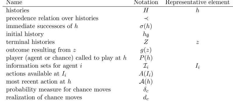
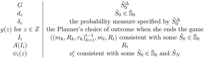
A mechanism is anextensive game form with consequences inX.9 This is an extensive game form where each terminal historyzresults in some outcomeg(z)∈X. We restrict attention to game forms with perfect recall10 and finite depth11. The full definition is familiar to most readers, so we relegate it to AppendixA.G denotes the set of all such game forms, with representative elementG. Useful notation is compiled in Table1.
Table 1: Notation for Extensive Game Forms
Name Notation Representative element
histories H h
precedence relation over histories ≺
immediate successors ofh σ(h)
initial history h∅
terminal histories Z z
outcome resulting fromz g(z) player (agent or chance) called to play ath P(h)
information sets for agenti Ii Ii
actions available atIi A(Ii) most recent action ath A(h) probability measure for chance moves δc realization of chance moves dc
We writeIi≺Ii′ if there exist historiesh∈Ii and h′ ∈Ii′ such that h≺h′. We write
Ii ≺h if there exists h′ ∈ Ii such that h′ ≺h. h≺Ii is defined symmetrically. We use
to denote the corresponding weak order.
Astrategy Si(·) chooses an action at every information set for agenti,Si(Ii)∈A(Ii). A strategy profile SN = (Si)i∈N specifies a strategy for each agent.
Atype-strategy Si(·) specifies a strategy for every type of agenti, whereSi(θi) denotes the strategy assigned to type θi. A type-strategy profile SN = (Si)i∈N specifies a type-strategy for each agent.
Let zG(h, S
N, δc) be the lottery over terminal histories that results in game form
G when we start from h and play proceeds according to (SN, δc). zG(h, SN, dc) is the
9By adopting this paradigm, we assume that the mechanism describes theentire strategic interaction
between the agents. For instance, after the mechanism has concluded, agent 1 cannot send money to agent 2, and agent 2 cannot throw a brick through agent 1’s window. Such post-game moves often imply that agents do not have dominant strategies, let alone obviously dominant strategies. Savage (1954) notes that “the use of modest little worlds, tailored to particular contexts, is often a simplification, the advantage of which is justified by a considerable body of mathematical experience with related ideas.”
10Ghasperfect recall if for any information setI
i, for any two historieshandh′inIi,ψi(h) =ψi(h′),
whereψ(h) is the experience of agentiat historyh(see Definition8).
11That is, for each game form, there exists some number k such that no history has more than
result of one realization of the chance moves under δc. We sometimes write this as
zG(h, Si, S−i, dc). LetuG
i (h, Si, S−i, dc, θi)≡ui(g(zG(h, Si, S−i, dc)), θi). This is the utility to agentiin game form G, when we start at history h, play proceeds according to (Si, S−i, dc), and the resulting outcome is evaluated according to preferencesθi.
Definition 1. Given Gand θi, Si isweakly dominant if: ∀Si′ :∀S−i :
Eδ
c[u G
i (h∅, Si′, S−i, dc, θi)]≤Eδc[u G
i (h∅, Si, S−i, dc, θi)] (2)
Letα(Si, Si′) be the set of earliest points of departure forSi andSi′. That is,α(Si, Si′) contains the information sets where Si and Si′ choose different actions, that can be on the path of play givenSi and givenSi′.
Definition 2 (Earliest Points of Departure). Ii ∈α(Si, Si′) if and only if:
1. Si(Ii)6=Si′(Ii)
2. There exist S−i, dc such thatIi≺zG(h∅, Si, S−i, dc).
3. There exist S−i, dc such thatIi≺zG(h∅, Si′, S−i, dc).
This definition can be extended to deal with mixed strategies12, but pure strategies suffice for our current purposes.
Definition 3. Given Gand θi, Si isobviously dominant if: ∀Si′ :∀Ii ∈α(Si, Si′) :
sup h∈Ii,S−i,dc
uGi (h, Si′, S−i, dc, θi)≤ inf h∈Ii,S−i,dc
uGi (h, Si, S−i, dc, θi) (3)
In words, Si is obviously dominant if, for any deviating strategy Si′, conditional on reaching any earliest point of departure, the best possible outcome underSi′ is no better than the worst possible outcome underSi.13
Compare Definition 1 and Definition 3. Weak dominance is defined using h∅, the history that begins the game. Consequently, if two extensive games have the same normal form, then they have the same weakly dominant strategies. Obvious dominance
12Three modifications are necessary: First, we change requirement 1 to be that both strategies specify
differentprobability measures atIi. Second, we adapt requirements 2 and 3 to hold forsome realization
of the mixed strategies. Finally, we include the recursive requirement, “There does not existIi′≺Iisuch
thatIi′∈α(Si, Si′).”
13Obvious dominance is related to conditional dominance (Shimoji and Watson,1998);S
iconditionally
dominatesS′iatIi if, for anyS−iconsistent with reachingIi, the payoff underSi′ is no better than the
is defined with histories that are in information sets that are earliest points of departure. Thus two extensive games with the same normal form may not have the same obviously dominant strategies.14 Switching to a direct revelation mechanism may not preserve obvious dominance, so the standard revelation principle does not apply.15
Weak dominance treats chance moves and other players asymmetrically. Suppose
G has a Bayes-Nash equilibrium, and we replace all the agents in N \1 with chance moves drawn from the Bayes-Nash equilibrium distribution. Then agent 1 has a weakly dominant strategy. By contrast, obvious dominance treats chance moves and other players symmetrically.
A choice rule is a functionf : ΘN →X. If we consider stochastic choice rules, then it is a functionf : ΘN →∆X.16
A solution concept C(·) is a set-valued function; for each G, it specifies a set of type-strategy profilesC(G), which may be an empty set.
Definition 4. (G,SN) C-implements f if:
1. SN ∈ C(G).
2. ∀θN ∈ΘN :f(θN) =g(zG(h∅,(Si(θi))i∈N, δc))
G C-implements f if there exists SN that satisfies the above requirements.
f isC-implementable if there exist (G,SN) that satisfy the above requirements.
Note that our concern is with weak implementation: We require that SN ∈ C(G), not {SN} = C(G). This is to preserve the analogy with canonical results for strategy-proofness, many of which assume weak implementation (Myerson, 1981; Saks and Yu, 2005).
Definition 5 (Strategy-Proof). SN ∈SP(G) if for all i and for allθi, Si(θi) is weakly
dominant.
14Two extensive games have the same reduced normal form if and only if they can be made identical
using a small set of elementary transformations (Thompson,1952;Elmes and Reny,1994). Which of these transformations does not preserve obvious dominance? Elmes and Reny (1994) propose three such transformations, INT, COA, and ADD, which preserve perfect recall. Brief inspection reveals that obvious dominance is invariant under INT and COA, but varies under ADD.
15Glazer and Rubinstein (1996) argue that extensive games can be easier to dominance-solve than
normal-form games, because backward induction provides guidance about the correct order to delete strategies. The standard revelation principle does not apply to their solution concept either.
16For readability, we generally suppress the latter notation, but the claims that follow hold for both
Definition 6 (Obviously Strategy-Proof). SN ∈ OSP(G) if for all i and for all θi, Si(θi) is obviously dominant.
A mechanism is weakly group-strategy-proof if there does not exist a coalition that could deviate and all bestrictly better off ex post.
Definition 7 (Weakly Group-Strategy-Proof). SN ∈WGSP(G) if there does not exist
a coalitionNˆ ⊆N, type profileθN, deviating strategiesSˆNˆ, non-coalition strategiesSN\Nˆ and chance movesdc such that: For all i∈Nˆ:
uGi (h∅,SˆNˆ, SN\Nˆ, dc, θi)> u G
i (h∅,SNˆ(θNˆ), SN\Nˆ, dc, θi) (4)
Obvious strategy-proofness implies weak group-strategy-proofness.17
Proposition 1. If SN ∈OSP(G), then SN ∈WGSP(G).
Proof. SupposeSN ∈/WGSP(G). Then there is a coalition ˆN with types ˆθNˆ that could
jointly deviate to strategies ˆSNˆ and all be strictly better off. FixSN\Nˆ anddc such that all agents in the coalition are strictly better off. Along the resulting terminal history, there is a first agentiin the coalition to deviate from Si(θi) to ˆSi. That first deviation happens at some information set Ii ∈ α(Si(θi),Sˆi). Agent i strictly gains from that deviation, soSN ∈/OSP(G).18
Corollary 1. If SN ∈OSP(G), then SN ∈SP(G).
Proposition1suggests a question: Is a choice rule OSP-implementable if and only if it is WGSP-implementable? Proposition 5shows that this is not so.
3.1 Cognitive limitations
In what sense is obvious dominance obvious? Intuitively, to see that Si′ is weakly dom-inated by Si, the agent must understand the entire function uG
i , and check that for all opponent strategy profilesS−i, the payoff from Si′ is no better than the payoff from Si. By contrast, to see that Si′ is obviously dominated by Si, the agent need only know the
range of the functions uG
i (·, Si′,· · ·) and uGi (·, Si,· · ·) at any earliest point of departure. Thus, obvious dominance can be recognized even if the agent has a simplified mental model of the world. We now make this point rigorously.
17Barber`a et al.(2016) note that “many well-known individually strategy-proof mechanisms are also
group strategy-proof, even if the latter is in principle a much stronger condition than the former.”
Definition 8. ψi(h) denotes i’s experience along history h; it is the sequence of in-formation sets where i was called to play, and the actions that i took, in order. We construct this by starting at h∅, and moving step-by-step through predecessors of h. At each h′ h, if P(h′) =i, then we add the current information set to the sequence. If i has just played an action ath′, then we add that action to the sequence.
We use Ψi to denote the set {ψi(h) |h∈H} ∪ψ∅, whereψ∅ is the empty sequence.19
We defineψi(Ii) :=ψi(h) |h∈Ii.
We define an equivalence relation between mechanisms. In words, G and G′ are
i-indistinguishable if there exists a bijection from i’s information sets and actions inG
onto i’s information sets and actions in G′, such that:
1. ψi is an experience inG iffψi’s image is an experience inG′.
2. Outcome x could follow experienceψi inGiff xcould follow ψi’s image in G′.
Definition 9. Take any G, G′ ∈ G, with information partitions Ii,Ii′ and experience
sets Ψi,Ψ′i. G and G′ are i-indistinguishable if there exists a bijection λG,G′ from
Ii∪A(Ii) toIi′∪A′(Ii′) such that:
1. ψi ∈Ψi iff λG,G′(ψi)∈Ψ′i
2. ∃z∈Z :g(z) =x, ψi(z) =ψi iff ∃z′∈Z′ :g′(z′) =x, ψi′(z′) =λG,G′(ψi)
where we use λG,G′(ψi) to denote the sequence produced by passing every element of ψi through λG,G′.
ForGandG′ that arei-indistinguishable, we defineλG,G′(Si) to be the strategy that,
given information set Ii′ inG′, plays λG,G′(Si(λ−G,G1 ′(Ii′))).
The next theorem states that obviously dominant strategies are the strategies that can be recognized as weakly dominant, by an agent who has this simplified mental model of the world.
Theorem 1. For any i, θi: Si is obviously dominant in G if and only if for every G′
that is i-indistinguishable from G, λG,G′(Si) is weakly dominant in G′.
The “if” direction permits a constructive proof. Suppose Si is not obviously domi-nant inG. Then there is some deviating strategySi′ and some earliest point of departure
Ii where the obvious dominance inequality does not hold. We construct a game form
19Mandating the inclusion of the empty sequence has the following consequence: By looking at the set
G′ that is i-indistinguishable fromG, such that, for some opponent strategies, if iplays
λG,G′(Si) then play proceeds according to the worst-case scenario (consistent with
reach-ing Ii), and if i deviates at λG,G′(Ii), then play proceeds according to some best-case
scenario (consistent with reaching Ii). The key is to find a general construction that always remains in the same equivalence class. The “only if” direction proceeds as fol-lows: Suppose there exists some G′ in the equivalence class of G, whereλG,G′(Si) is not
weakly dominant. There exists some earliest information set inG′ whereicould gain by deviating. We then useλ−G,G1 ′ to locate an information set inG, and a deviationSi′, that
do not satisfy the obvious dominance inequality. AppendixBprovides the details. One interpretation of Theorem1is that obviously dominant strategies are those that can be recognized as dominant given only a partial description of the game form.
Another interpretation of Theorem 1 is that obviously dominant strategies are ro-bust to local misunderstandings. Suppose an agent could mistake any G for any i -indistinguishableG′. He has some belief about how his opponents are playing inG′, and best responds to that (mistaken) belief. For instance, when faced with a second-price auction, he could believe that he faces a third-price auction20, in which case bidding above his value is a best response to the (symmetric) Nash equilibrium opponent strate-gies (Kagel and Levin, 1993). When is his (true) dominant strategy still in his set of best responses, for any such local mistake? By Theorem1, this holds if and only if it is obviously dominant.
Many solution concepts in behavioral game theory specify that agents understand the game form, but best-respond to mistaken beliefs about opponent strategies.21 Since a dominant strategy is always a best response, such theories predict no mistakes in strategy-proof mechanisms.22 Obvious dominance captures misunderstandings about the game form, and is thus orthogonal to these theories.
3.2 Supported by bilateral commitments
Suppose the following augmented game form ˜G with consequences in X: As before we have a set of agentsN, outcomes X, and preference profilesQi∈NΘi. However, there is one player in addition to N: Player 0, the Planner.
20In both second-price and third-price auctions, the bidder submits a sealed bid. For any sealed bid,
either he receives the object and pays a price less than or equal to his bid, or does not receive the object and makes no payments. Thus, both mechanisms arei-indistinguishable.
21Such concepts include level-k equilibrium (Stahl and Wilson, 1994, 1995; Nagel, 1995), cognitive
hierarchy equilibrium (Camerer et al., 2004), cursed equilibrium (Eyster and Rabin, 2005; Esponda,
2008), and analogy-based expectation equilibrium (Jehiel,2005).
The Planner has an arbitrarily rich message spaceM. At the start of the game, each agenti∈N privately observesθi. Play proceeds as follows:
1. The Planner chooses one agenti∈N and sends a query m∈M, along with a set of acceptable repliesR⊂M.23
2. iobserves (m, R), and chooses a reply r∈R.
3. The Planner observesr.
4. The Planner either selects an outcomex∈X, or chooses to send another query.
(a) If the Planner selects an outcome, the game ends.
(b) If the Planner chooses to send another query, go to Step 1.
For i∈N,i’s type-strategy specifies what reply to give, as a function of his prefer-ences, the past sequence of queries and replies between him and the Planner, and the current (m, R). That is:
˜
Si(θi,(mk, Rk, rk)t−k=11, mt, Rt)∈Rt (5)
Analogously, a strategy ˜Si depends on ((mk, Rk, rk)kt−=11, mt, Rt), but not on θi. We use ˜Sθi
i to denote the strategy played by typeθiof agenti. We abbreviate (˜Sθii)i∈N ≡S˜ θN N . ˜
S0 denotes a pure strategy for the Planner; where S0 denotes the set of all pure
strategies. We restrict the Planner to send only finitely many queries.
The standard full commitment paradigm is equivalent to allowing the Planner to commit to a unique ˜S0∈S0 (or some probability measure over S0). Instead, we assume
that for each agent, the Planner can commit to a subset ˆSi
0 ⊆S0 that is measurable with
respect to that agent’s observations in the game.
This is formalized as follows: Each ( ˜S0,S˜N) results in some observationoi ≡(oCi , oXi ), consisting of a communication sequence between the Planner and agenti,oC
i = (mk, Rk, rk)Tk=1 forT ∈N, as well as some outcome oX
i ∈X.24 Oi is the set of all possible observations (for agent i). We define φi :S0×SN → Oi, where φi( ˜S0,S˜N) is the unique observation resulting from ( ˜S0,S˜N). Next we define, for any ˆS0 ⊆S0:
Φi(ˆS0)≡ {oi | ∃S˜0 ∈Sˆ0 :∃S˜N :oi =φi( ˜S0,S˜N)} (6)
23This game could be made simpler without altering Theorem2; the Planner could send only a set of
acceptable repliesR⊂M. Any information contained in the query could simply be ‘written into’ every acceptable reply. However, distinguishing queries and replies makes the exposition more intuitive.
For any ˆOi⊆ Oi:
Φ−i 1( ˆOi)≡ {S0˜ | ∀S˜N :φi( ˜S0,S˜N)∈Oˆi} (7)
Definition 10. Sˆ0 is i-measurable if there exists Oˆi such that:
ˆ
S0 = Φ−1
i ( ˆOi) (8)
Intuitively, thei-measurable subsets ofS0are those such that, if the Planner deviates,
then there exists an agent strategy profile such that agent idetects the deviation; that is, i has an observation that is not compatible with any strategy in the promised set. Formally, the i-measurable subsets of S0 are the σ-algebra generated by Φi (where we
impose the discreteσ-algebra on Oi).25
Definition 11. A mixed strategy of finite length over Sˆ0 specifies a probability
measure over a subset ¯S0 ⊆Sˆ0 such that: There exists k∈Nsuch that: For all S0˜ ∈¯S0
and all S˜N: ( ˜S0,S˜N) results in the Planner sending k or fewer total queries.
We use ∆ˆS0 to denote the mixed strategies of finite length over ˆS0. ˜S∆
0 denotes an
element of such a set.
Definition 12. A choice rule f is supported by bilateral commitments (ˆSi
0)i∈N if
1. For all i∈N: ˆSi0 isi-measurable.
2. There exist S˜0∆, and S˜N such that:
(a) For all θN: ( ˜S0∆,S˜NθN) results in f(θN).
(b) S˜0∆∈∆Ti∈NˆSi
0
(c) For alli∈N,θi, S˜N\i′ ,S˜0∆′ ∈∆ˆSi0: S˜θii is a best response to( ˜S0∆′,S˜N\i′ ) given
preferences θi.
Requirement 2.a is that the Planner’s mixed strategy and the agent’s pure strategies result in the (distribution over) outcomes required by the choice rule. Requirement 2.b
is that the Planner’s strategy is a (possibly degenerate) mixture over pure strategies
25Notice that an observation for playeriis simply a sequence of messages and responses, followed by
compatible withevery bilateral commitment.26 2.cis that each agenti’s assigned strat-egy is weakly dominant, when we consider the Planner as a player restricted to playing mixtures over strategies in ˆSi
0.
“Supported by bilateral commitments” is just one of many partial commitment regimes. This one requires that the commitment offered to each agent is measurable with respect to events that he can observe. In reality, contracts are seldom enforceable unless each party can observe breaches. Thus, “supported by bilateral commitments” is a natural case to study.
Theorem 2. f is OSP-implementable if and only if there exist bilateral commitments
(ˆSi
0)i∈N that support f.
The intuition behind the proof is as follows: A bilateral commitment ˆSi
0 is essentially
equivalent to the Planner committing to ‘run’ only games in some i-indistinguishable equivalence class of G. Consequently, we can find a set of bilateral commitments that support fy if and only if we can find some (G,SN) such that, for every i, for every θi, for every G′ that isi-indistinguishable fromG,λG,G′(Si(θi)) is weakly dominant in G′.
By Theorem1, this holds if and only if fy is OSP-implementable. AppendixBprovides the details.
3.3 The pruning principle
When seeking SP-implementation, we can without loss of generality restrict attention to the class of direct revelation mechanisms, by the revelation principle. The standard revelation principle does not hold for OSP mechanisms. As the second-price auction illustrates, there exist OSP-implementable choice rules that cannot be implemented via a direct revelation mechanism.
However, there is a weaker principle that substantially simplifies the analysis. Here we define the pruning of a mechanism with respect to a type-strategy profile. If, for all type profiles, a history is never reached, then we delete that history (and redefine the other parts of the tuple so that what remains is well-formed).
Definition 13(Pruning). Take anyG=hH,≺, A,A, P, δc,(Ii)i∈N, gi, andSN. P(G,SN)≡
hH,˜ ≺˜,A,˜ A˜,P ,˜ δ˜c,(˜Ii)i∈N,g˜i is the pruningofGwith respect to SN, constructed as
fol-lows:
1. H˜ ={h∈H | ∃θN :∃dc : hzG(h∅,(Si(θi))i∈N, dc)}
26This requirement prevents the Planner from extracting arbitrary information by making promises
2. For all i, if Ii ∈ Ii then (Ii∩H˜)∈I˜i.27
3. ( ˜≺,A,˜ A˜,P ,˜ δ˜c,˜g) are (≺, A,A, P, δc, g) restricted to H.˜
It turns out that, if some mechanism OSP-implements a choice rule, then the pruning of that mechanism with respect to the equilibrium strategies OSP-implements that same choice rule. Thus, while we cannot restrict attention to direct revelation mechanisms, we can restrict attention to ‘minimal’ mechanisms, such that no histories are off the path of play. This is used both in this paper and in the subsequent literature28to state clean results.
Proposition 2 (The Pruning Principle). Let G˜ ≡ P(G,SN), and S˜N be SN restricted
toG. If˜ (G,SN) OSP-implements f, then ( ˜G,S˜N) OSP-implements f.
4
Applications
4.1 Binary Allocation Problems
We now consider a canonical environment, (N, X,ΘN,(ui)i∈N). LetY ⊆2N be the set of feasible allocations, with representative element y ∈ Y. An outcome consists of an allocationy∈Y and a transfer for each agent,X=Y ×Rn. t≡(ti)i∈N denotes a profile
of transfers.
Preferences are quasilinear. ΘN =Qi∈NΘi, where Θi = [θi, θi], for 0≤θi < θi <∞. Forθi∈Θi,
ui(θi, y, t) = 1i∈yθi+ti (9)
For instance, in a private value auction with unit demand, i∈y if and only if agent
i receives at least one unit of the good under allocation y. In a procurement auction,
i∈y if and only if idoes not incur costs of provision under allocationy. θi is agent i’s cost of provision (equivalently, benefit of non-provision). In a binary public goods game,
Y ={∅, N}.
An allocation rule is a function fy : Θ →Y. A choice rule is thus a combination of an allocation rule and a payment rule, f = (fy, ft), where ft : Θ → Rn. Similarly, for each game form G, we disaggregate the outcome function, g= (gy, gt). In this part, we concern ourselves only with deterministic allocation rules and payment rules, and thus suppress notation involvingδc and dc.
27Note that the initial historyh
∅is distinct from the empty set. That is to say, (Ii∩H˜) =∅doesnot
entail that{h∅} ∈I˜i.
Definition 14. An allocation rule fy is C-implementable if there exists ft such that (fy, ft)isC-implementable. GC-implementsfy if there existsftsuch thatGC-implements (fy, ft)
In a binary allocation problem,fyis SP-implementable if and only iffyis monotone.29 This result is implicit inSpence (1974) andMirrlees (1971), and is proved explicitly in Myerson (1981).30 Moreover, if an allocation rule fy is SP-implementable, then the accompanying transfer rule ftis essentially unique.
ft,i(θi, θ−i) =−1i∈fy(θ)inf{θ ′
i |i∈fy(θi′, θ−i)}+ri(θ−i) (10)
where ri is some arbitrary function of the other agents’ preferences. This follows easily by arguments similar to those inGreen and Laffont(1977) andHolmstr¨om(1979). In this standard environment, what happens when we require OSP-implementation? In particular, what restrictions does OSP-implementation place on the transfer rules and the extensive game form?
In binary allocation problems, every OSP mechanism is essentially a personal-clock auction. It is personal in two respects: Firstly, the clock price and closing rule could vary across agents. Secondly, the clock price could be associated with different consequences for different agents. The full statement of the definition is novel, but we will build it out of familiar parts.
Consider how the ascending auction appears to a single bidder: At each point, there is a ‘going transfer’ associated with being in the allocation (winning the object). The agent either playsquit orcontinue; if he playsquit, then he is out of the allocation and makes no payments. If he playscontinue, then either he is in the allocation and has the going transfer, or the going transfer falls (the going price rises) and he faces the same decision again.
We can generalize this procedure a bit, while still ensuring that the agent has an obviously dominant strategy. The going transfer could fall in any increments, and how much it falls could depend on other agents’ actions. The transfer associated with being out of the allocation could be non-zero, as long as it is some (known) fixed amount. Even if the agent choosescontinue, we could sometimes mandate that he quits, in which case he is out of the allocation (and receives the fixed transfer). The agent need not choose
29f
y is monotone if for alli, for allθ−i, 1i∈fy(θi,θ−i) is weakly increasing inθi.
30These monotonicity results for are for weak SP-implementation rather than full SP-implementation
implementation. Weak SP-implementation requires SN ∈ SP(G). Full SP-implementation requires
SN= SP(G). There are monotone allocation rules for which the latter requirement cannot be satisfied.
For example, suppose two agents with unit demand. Agent 1 receives one unit iff v1 > .5. Agent 2
betweencontinue andquitat every information set; he need only be offered a choice when the going transfer strictly falls. There could be multiple actions thatquit, all having the same consequence for him.31 There could be multiple actions that continue, provided that the going transfer will not fall in future and at least one such action guarantees that he is in the allocation. The agent could receive arbitrary information about the history of play. We call this generalized procedure In-Transfer Falls.
Consider how a descending-price procurement auction appears to a single supplier (holding one unit of an indivisible good): At each point, there is a ‘going transfer’ associated with being out of the allocation. The agent either plays quit orcontinue; if he plays quit, then he is in the allocation (keeps the good) and receives nothing. If he plays continue, then either he is out of the allocation (sells the good) and receives the going transfer, or the going transfer falls and he faces the same decision again. Notice that now the transfer associated with being in the allocation is fixed and the transfer associated with being out of the allocation falls monotonically. We could generalize this in the same ways as before, and call the resulting procedureOut-Transfer Falls.
In apersonal-clock auction, starting from any point an agent first has a non-singleton information set, that agent either facesIn-Transfer Falls orOut-Transfer Falls.
Definition 15. G is a personal-clock auction if, for every i ∈N, at every earliest information setIi∗ such that |A(Ii∗)|>1:
1. Either (In-Transfer Falls): There exists a fixed transfer ¯ti ∈R, a going transfer ˜
ti:{Ii |Ii∗Ii} →R, and a set of ‘quitting’ actions Aq such that:
(a) For all z where Ii∗≺z:
i. Either: i /∈gy(z) and gt,i(z) = ¯ti.
ii. Or: i∈gy(z) and
gt,i(z) = inf Ii:Ii∗Ii≺z
˜
ti(Ii) (11)
(b) For all a∈Aq, for all z such that a∈ψi(z): i /∈gy(z)
(c) Aq∩A(I∗ i)6=∅.
(d) For all Ii′, Ii′′∈ {Ii |Ii∗ Ii}:
i. IfIi′ ≺Ii′′, then t˜i(Ii′)≥˜ti(I′′ i).
ii. If Ii′ ≺ Ii′′, ˜ti(Ii′) > t˜i(Ii′′), and there does not exist Ii′′′ such thatIi′ ≺
Ii′′′≺Ii′′, then Aq∩A(I′′ i)6=∅.
31Although they could affect what happens to other agents - it is incentive compatible for the agent
iii. IfIi′ ≺Ii′′ and ˜ti(Ii′)>˜ti(Ii′′), then |A(Ii′)\Aq|= 1.
iv. If |A(Ii′)\Aq|>1, then there exists a∈A(I′
i) such that: For all z such
that a∈ψi(z): i∈gy(z).
2. Or (Out-Transfer Falls): As above, but we substitute every instance of “i ∈
gy(z)” with “i /∈gy(z)” and vice versa.
Notice what this definition does not require. The going transfer need not be equal across agents. Whether and how much one agent’s going transfer changes could depend on other agents’ actions. Some agents could face In-Transfer Falls, and other agents could face Out-Transfer Falls (a two-sided clock auction).32 Which procedure an agent faces could even depend on other agents’ past actions.
Theorem 3. If(G,SN)OSP-implements fy, thenP(G,SN)is a personal-clock auction.
If G is a personal-clock auction, then there exist SN and fy such that (G,SN)
OSP-implementsfy.
For any normal-form mechanism, there are typically many equivalent extensive forms. The theory of mechanism design seldom provides general criteria to choose between them. In binary allocation problems, obvious dominance pins down many extensive-form details of the ascending auction, and provides an answer to the question, “Why are ascending auctions so common?”
4.2 Top Trading Cycles
We now produce an impossibility result in a classic matching environment (Shapley and Scarf,1974). There arenagents in the market, each endowed with an indivisible good. An agent’s type is a vectorθi ∈Rn. ΘN is the set of allnbynmatrices of real numbers. An outcome assigns one object to each agent. If agent i is assigned object k, he has utilityθki. There are no money transfers.
Given preferencesθand agentsR⊆N, atop trading cycle is a set∅ ⊂R′ ⊆Rwhose members can be indexed in a cyclic order:
R′ ={i1, i2, . . . , ir=i0} (12)
such that each agent ik likes ik+1’s good at least as much as any other good in R.
FollowingRoth(1982), we assume that the algorithm in question has an arbitrary, fixed way of resolving ties.
32Loertscher and Marx(2017) investigate two-sided clock auctions that are prior-free, asymptotically
Definition 16. f is a top trading cycle rule if, for all θ, f(θ) is equal to the output of the following algorithm:
1. Set R1 :=N
2. For l= 1,2, , . . .:
(a) Choose some top trading cycle R′⊆Rl.
(b) Carry out the indicated trades.
(c) Set Rl+1 :=Rl\R′.
(d) Terminate ifRl+1=∅.
The above algorithm is of economic interest, because it finds a core allocation in an economy with indivisible goods (Shapley and Scarf,1974).
Proposition 3. If f is a top trading cycle rule, then there existsGthat SP-implements f. (Roth, 1982)
Proposition 4. If f is a top trading cycle rule, then there exists G that WGSP-implementsf. (Bird, 1984)
Proposition 5. If f is a top trading cycle rule and n≥3, then there does not exist G that OSP-implements f.
Proof. OSP-implementability is a hereditary property of functions. That is, iff is OSP-implementable given domain ΘN, then the subfunctionf′ =f with domain Θ′N ⊆ΘN is OSP-implementable. Thus, to prove Proposition 5, it suffices to produce a subfunction that is not OSP-implementable.
Consider the following subset Θ′N ⊂ ΘN. Take agents a, b, c, with endowed goods
A, B, C. ahas only two possible types,θa andθa′, such that
EitherB ≻aC≻aA≻a. . .
orC ≻aB≻aA≻a. . .
(13)
We make the symmetric assumption for band c.
Suppose not, and supposeB ≻aC. Ifachooses the action corresponding toB ≻aC, and faces opponent strategies corresponding to C ≻b A and B ≻c A, then a receives goodA. Ifachooses the action corresponding toC≻aB, and faces opponent strategies corresponding A≻c B, then areceives good C. Thus, it is not an obviously dominant strategy to choose the action corresponding toB ≻aC. Soacannot be the first to have a non-singleton action set.
By symmetry, this argument applies to b and c as well. So all of the action sets for
a,b, and c are singletons, andGdoes not OSP-implement f′, a contradiction.
Proposition 5 implies that the OSP-implementable choice rules are not identical to the WGSP-implementable choice rules.
5
Laboratory Experiment
Are obviously strategy-proof mechanisms easier for real people to understand? The following laboratory experiment provides a straightforward test: We compare pairs of mechanisms that implement the same choice rule. One mechanism in each pair is SP, but not OSP. The other mechanism is OSP. Standard game theory predicts that both mechanisms will produce the same outcome. We are interested in whether subjects play the dominant strategy at higher rates under OSP mechanisms.
5.1 Experiment Design
The experiment is an across-subjects design, comparing three pairs of games. There are four players in each game.
For the first pair, we compare the second-price auction (2P) and the ascending clock auction (AC). In both these games, subjects bid for a money prize. Subjects have induced affiliated private values; if a subject wins the prize, he earns an amount equal to the value of the prize, minus his payments from the auction. For each subject, his value for the prize is equal to a group draw plus a private adjustment. The group draw is uniformly distributed between $10 and $110. The private adjustment is uniformly distributed between $0 and $20. All money amounts in these games are in 25-cent increments. Each subject knows his own value, but not the group draw or the private adjustment.33
33I use affiliated private values for two reasons. First, in strategy-proof auctions with independent
2Pis SP, but not OSP. In2P, subjects submit their bids simultaneously. The highest bidder wins the prize, and makes a payment equal to the second-highest bid. Bids are constrained to be between $0 and $150.34
AC is OSP. In AC, the price starts at a low value (the highest $25 increment that is below the group draw), and counts upwards, up to a maximum of $150. Each bidder can quit at any point.35 When only one bidder is left, that bidder wins the object at the current price.
Previous studies comparing second-price auctions to ascending clock auctions have small sample sizes, given that when the same subjects play a sequence of auctions, these are plainly not independent observations. Kagel et al.(1987) compare 2 groups playing second-price auctions to 2 groups playing ascending clock auctions. Harstad (2000) compares 5 groups playing second-price auctions to 3 groups playing ascending clock auctions. (The comparison is not the main goal of either experiment.) Other studies find similar results for second-price auctions (Kagel and Levin, 1993) and for ascending clock auctions (McCabe et al.,1990), but these do not directly compare the two formats with the same value distribution and the same subject pool. When we compare2P and AC, we can see this as a high-powered replication of Kagel et al. (1987), since we now observe 18 groups playing2P and 18 groups playing AC.36
For the second pair, we compare the second-price plus-X auction (2P+X) and the ascending clock plus-Xauction (AC+X). Subjects’ values are drawn as before. However, there is an additional random variableX, which is uniformly distributed between $0 and $3. Subjects are not told the value ofX until after the auction.
2P+X is SP, but not OSP. In 2P+X, subjects submit their bids simultaneously. The highest bidder wins the prize if and only if his bid exceeds the second-highest bid plus X. If the highest bidder wins the prize, then he makes a payment equal to the second-highest bid plus X. Otherwise, no agent wins the prize, and no payments are made. In this game, it is a dominant strategy to submit a bid equal to your value.
AC+Xis OSP. InAC+X, the price starts at a low value (the highest $25 increment that is below the group draw), and counts upwards. Each bidder can quit at any point.37 When only one bidder is left, the pricecontinues to rise for anotherX dollars, and then
34In both2PandAC, if there is a tie for the highest bid, then no bidder wins the object. 35During the auction, each bidder observes the number of active bidders.
36I am not aware of any previous laboratory experiment that directly compares second-price and
ascending clock auctions, holding constant the value distribution and subject pool, with more than five groups playing each format.
37As in AC, each bidder observes the number of active bidders. However, if the number of active
freezes. If the highest bidder keeps bidding until the price freezes, then she wins the prize at the final price. Otherwise, no agent wins the prize and no payments are made. In this game, it is an obviously dominant strategy to keep bidding if the price is strictly below your value, and quit otherwise.
Some subjects might find2P or AC familiar, since such mechanisms occur in some natural economic environments. Differences in subject behavior might be caused by dif-ferent degrees of familiarity with the mechanism. 2P+X and AC+X are novel mech-anisms that subjects are unlikely to find familiar. 2P+X and AC+X can be seen as perturbations of2PandAC; the underlying choice rule is made more complex while pre-serving the SP-OSP distinction. Thus, comparing2P+XandAC+Xindicates whether the distinction between SP and OSP mechanisms holds for novel and more complicated auction formats.
In the third pair of games, subjects may receive one of four common-value money prizes. The four prize values are drawn, uniformly at random and without replacement, from the set {$0.00,$0.25,$0.50,$0.75,$1.00,$1.25}. Subjects observe the values of all four prizes at the start of each game.
In a strategy-proof random serial dictatorship (SP-RSD), subjects are informed of their priority score, which is drawn uniformly at random from the integers 1 to 10. They then simultaneously submit ranked lists of the four prizes. Players are processed sequentially, from the highest priority score to the lowest. Ties in priority score are broken randomly. Each player is assigned the highest-ranked prize on his list, among the prizes that have not yet been assigned. It is a dominant strategy to rank the prizes in order of their money value. SP-RSDis SP, but not OSP.38
In an obviously strategy-proof random serial dictatorship (OSP-RSD), subjects are informed of their priority score. Players take turns, from the highest priority score to the lowest. When a player takes his turn, he is shown the prizes that have not yet been taken, and picks one of them. It is an obviously dominant strategy to pick the available prize with the highest money value.
SP-RSD and OSP-RSD differ from the auctions in several ways. The auctions are private-value games of incomplete information, whereas SP-RSD and OSP-RSD are common-value games of complete information. In the auctions, subjects face two sources of strategic uncertainty: They are uncertain about their opponents’ valuations, and they are uncertain about their opponents’ strategies (a function of valuations). By contrast, in SP-RSD and OSP-RSD, subjects face no uncertainty about their
38SP-RSDis SP, but not OSP since, if a player swaps the order of the highest and second-highest
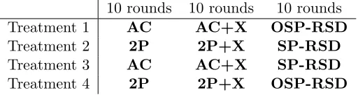
Table 2: Mechanisms in each treatment
10 rounds 10 rounds 10 rounds
Treatment 1 AC AC+X OSP-RSD
Treatment 2 2P 2P+X SP-RSD
Treatment 3 AC AC+X SP-RSD
Treatment 4 2P 2P+X OSP-RSD
opponents’ valuations.
Unlike the auctions, SP-RSD and OSP-RSD are constant-sum games, such that one player’s action cannot affect total player surplus. Any effect that persists in both the auctions and the serial dictatorships is difficult to explain using social preferences, since such theories typically make different predictions for constant-sum and non-constant-sum games. Thus, in comparingSP-RSDandOSP-RSD, we test whether the SP-OSP distinction has empirical support in mechanisms that are very different from auctions.
At the start of the experiment, subjects are randomly assigned into groups of four. These groups persist throughout the experiment. Consequently, each group’s play can be regarded as a single independent observation in the statistical analysis.
Each group either plays 10 rounds of AC, followed by 10 rounds of AC+X, or plays 10 rounds of 2P, followed by 10 rounds of 2P+X.39At the end of each round, subjects are shown the auction result, their own profit from this round, the winning bidder’s profit from this round, and the bids (in order from highest to lowest). Notice that subjects have 10 rounds of experience with a standard auction, before being presented with its unusual+X variant. Thus, the data from +Xauctions record moderately experienced bidders grappling with a new auction format.
Next, groups are re-randomized into either 10 rounds of OSP-RSDor 10 rounds of SP-RSD. At the end of each round, subjects see which prize they have obtained, and whether their priority score was the highest, or second-highest, and so on.
Table2 summarizes the design. Subjects had printed copies of the instructions, and the experimenter read aloud the part pertaining to each 10-round segment just before that segment began. The instructions (correctly) informed subjects that their play in earlier segments would not affect the games in later segments. The instructions did not mention dominant strategies or provide recommendations for how to play, so as to prevent confounds from the experimenter demand effect. Instructions for both SP and
39If a stage game with dominant strategies is repeated finitely many times, then the resulting repeated
OSP mechanisms are of similar length and similar reading levels40, and can be found in the online appendix.
In every SP mechanism, each subject had 90 seconds to make his choice. Each subject could revise his choice as many times as he desired during the 90 seconds, and only his final choice would count. For OSP mechanisms, mean time to completion was 113.0 seconds in AC, 121.4 seconds in AC+X, and 40.5 seconds in OSP-RSD. However, the rules of the OSP mechanisms imply that not every subject was actively choosing throughout that time.
5.2 Administrative details
Subjects were paid $20 for participating, in addition to their profits or losses from every round of the experiment. On average, subjects made $37.54, including the participation payment. Subjects who made negative net profits received just the $20 participation payment.
I conducted the experiment at the Ohio State University Experimental Economics Laboratory in August 2015, using z-Tree (Fischbacher,2007). I recruited subjects from the student population using an online system (Greiner, 2015). I administered 16 ses-sions, where each session involved 1 to 3 groups. Each session lasted about 90 minutes. In total, the data include 144 subjects in 36 groups of 4 (with 9 groups in each treatment).41
5.3 Statistical Analysis
The data include 4 different auction formats, with 180 auctions per format, for a total of 720 auctions.42
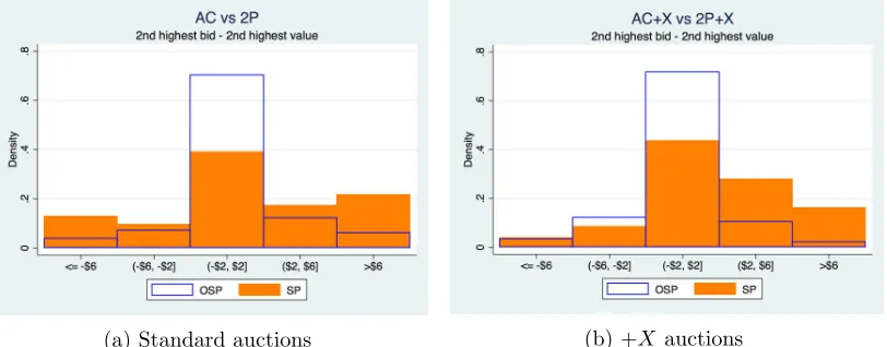
One natural summary statistic for each auction is the difference between the second-highest bid and the second-second-highest value. This is, equivalently, the difference between that auction’s closing price, and the closing price that would have occurred if all bidders played the dominant strategy. Figure 2a displays histograms of the second-highest bid minus the second-highest value, for AC and 2P. Figure 2b does the same for AC+X and 2P+X. If all agents are playing the dominant strategy in an auction, then the histogram for that auction will be a point mass at zero.
40Both sets of instructions are approximately at a fifth-grade reading level according to the
Flesch-Kincaid readability test, which is a standard measure for how difficult a piece of text is to read (Kincaid et al.,1975).
41In two cases, network errors caused crashes which prevented a group from continuing in the
experi-ment. I recruited new subjects to replace these groups.
42In 2 out of 720 auctions, computer errors prevented bidders from correctly entering their bids. We
(a) Standard auctions (b) +X auctions
Figure 2: Histogram: 2nd-highest bid minus 2nd-highest value
There is a substantial difference between the empirical distributions for OSP and SP mechanisms. If we choose a random auction from the data, how likely is it to have a closing price within $2.00 of the equilibrium price? An auction is 31 percentage points more likely to have a closing price within $2.00 of the equilibrium price underAC(OSP) compared to 2P (SP). An auction is 28 percentage points more likely to have a closing price within $2.00 of the equilibrium price under AC+X (OSP) compared to 2P+X (SP). Closing prices under2P+X are systematically biased upwards (p=.0031)43.
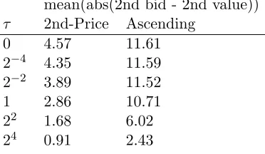
Table3displays the mean absolute difference between the second-highest bid and the second-highest value, for the first 5 rounds and the last 5 rounds of each auction. This measures the magnitude of errors under each mechanism. (Alternative measures of errors are in AppendixC.) Errors are systematically larger under SP than under OSP, and this difference is significant in both the standard auctions and the novel+Xauctions, and in both early and late rounds. To build intuition for effect sizes, consider that the expected profit of the winning bidder in 2P and AC is about $4.00 (given dominant strategy play). Thus, the average errors under2P are larger than the theoretical prediction for total bidder surplus.
There is some evidence of learning in 2P; errors are smaller in the last five rounds compared to the first five rounds (p=.045, paired t-test). For the other three auction formats, there is no significant evidence of learning.44
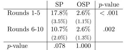
To compare subject behavior under SP-RSDand OSP-RSD, we compute the
pro-43For each group, we take the mean difference between the second-highest bid and the second-highest
value. This produces one observation per group playing2P+X, for a total of 18 observations, and we use at-test for the null that these have zero mean.
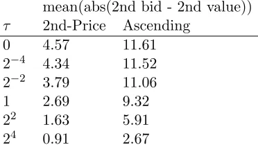
Table 3: mean(abs(2nd bid - 2nd value))
Format Rounds SP OSP p-value
Auction
1-5 8.04 3.19 .006
(1.25) (1.05)
6-10 4.99 1.77 .016
(1.18) (0.33)
+X Auction
1-5 3.99 1.83 .006
(0.60) (0.41)
6-10 3.69 1.29 .017
(0.87) (0.33)
[image:30.612.209.405.333.414.2]For each group, we take the mean absolute difference over each 5-round block. We then compute standard errors counting each group’s 5-round mean as a single observation. (18 observations per cell, standard errors in parentheses.) p-values are computed using a two-samplet-test, allowing for unequal variances. Other empirical strategies yield similar results; see AppendixCfor details.
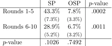
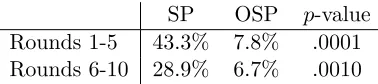
Table 4: Proportion of serial dictatorships not ending in dominant strategy outcome
SP OSP p-value Rounds 1-5 43.3% 7.8% .0002
(7.3%) (3.3%)
Rounds 6-10 28.9% 6.7% .0011
(5.2%) (3.2%)
p-value .1026 .7492
For each group, for each 5-round block, we record the error rate. We then compute standard errors counting each group’s observed error rate as a single observation. (18 observations per cell, standard errors in parentheses.) When comparing SP to OSP, we compute p-values using a two-samplet-test, allowing for unequal variances. (Alternative empirical strategies yield similar results. See AppendixC
for details.) When comparing early to late rounds of the same game, we computep-values using a paired
t-test.
portion of games that do not end in the dominant strategy outcome. UnderSP-RSD, 36% of games do not end in the dominant strategy outcome. Under OSP-RSD, 7% of games do not end in the dominant strategy outcome. Table 4 displays the empirical frequency of non-dominant strategy outcomes, by format and by 5-round blocks. De-viations from the dominant strategy outcome happen more frequently under SP-RSD than under OSP-RSD, and these differences are highly significant in both early and late rounds.