Munich Personal RePEc Archive
Disentanglement of natural interest rate
shocks and monetary policy shocks nexus
Kurovskiy, Gleb
12 December 2019
Online at
https://mpra.ub.uni-muenchen.de/97547/
Disentanglement of natural interest rate shocks and monetary
policy shocks nexus
Gleb Kurovskiy
draft
December 12, 2019
Abstract
This paper proposes a novel two-step identification procedure of natural interest rate shocks.
Al-together, monetary policy and natural interest shocks explain about 90% of total inflation dynamics.
The paper exploits (J.E. Arias et al., 2019) procedure, which allows getting canonical impulse response
functions to monetary policy shocks. I find no evidence of price and output puzzles. The estimated
natural interest rate declines from 2015 to 2019 years. Furthermore, Bank of Russia follows mandate
and reacts to inflation in monetary policy feedback rule, while does not respond to output fluctuations.
Keywords: SVAR, monetary policy, natural interest rate, Russia
Introduction and literature review
The impact of monetary policy on the real part of economy has been in the focus of researchers’
attention for almost five decades. The question renewed its importance when the world’s most influential
central banks switched to inflation targeting regime. There are two competing strategies on how to achieve
the inflation target. The first strategy is to forecast inflation ahead, compare it with a desired target,
and manipulate the monetary policy rate to keep inflation on target. The second strategy is to estimate
the natural interest rate and keep the policy rate at the natural level. This paper shows how these two
strategies may coexist and explains how monetary policy shocks may be estimated simultaneously with
the natural interest rate within one model.
The first approach implies, if central banks economists estimate the delay of the policy instrument
effect on inflation and economic activity to be two years. If central banks experts predict inflation going
above the inflation target in two years, then central banks would hike the policy rate to shrink inflation
in two years and return it to target. However, not all policy rate hikes lead to a decrease in inflation
or economic activity but only those hikes that are unexpected to economic agents. In the present paper,
I follow Christiano, L. J. et al., (1999) and define monetary policy shocks as unanticipated to economic
agents changes (or unchanges) in the policy rate. One of the dominating methods of obtaining structural
shocks is the identification of structural vector autoregression models (SVAR). For an extensive review of
identification techniques, I refer to papers by Christiano, L. J. et al. (1999) and Ramey, V. A. (2016). The
problem with such an approach is double uncertainty around the estimates of monetary policy shocks and
predictions of macroeconomic variables.
The second approach impies, central banks experts find it useful to conduct their monetary policy via
monetary stance (the difference between the policy rate and the natural interest rate). I define the natural
interest rate in the same way as Laubach, T. and Williams, J. C. (2003), as a real interest rate when the
output is equal to its natural level and inflation is equal to its target. Central bankers compare the natural
interest rate with the policy rate. If the natural rate is higher than the policy rate, then the output is
higher than its potential level or/and the inflation is higher than its target. Therefore, central banks should
hike the policy rate to stabilize inflation and output to its potential and target levels. However, there are
at least two problems related to this approach.
Firstly, the gap could never close due to nominal wage and price rigidities (Amato 2005). Secondly,
a natural interest rate is an unobservable variable, and natural rate estimates are highly imprecise. “It
is a well-known fact that estimates of the natural rate of interest, commonly referred to as r*, are highly
the US natural rate could currently be anywhere between -3% and +5%” speech by Benoˆıt Cœur´e 17
September 2018 at ECB. To evaluate monetary policy stance, central bank economists need to estimate
natural interest rate and forecast factors which influence a natural interest rate future dynamics. The
dominating part of a natural interest factors come from the real part of the economy.
In Ramsey model (Ramsey, 1928) of neoclassical growth, the natural interest rate depends on the
intertemporal substitution, population growth and technological growth. The other factors could be the
potential output, fiscal policy, demography (T. Laubach and J. C. Williams, 2003); (Holston, K., 2017);
(Orphanides, A., and Williams, J. C., 2002). Therefore, to conduct monetary policy central bankers should
predict the factors of a natural interest rate and determine how these factors influence a natural rate. Supply
shocks, technological shocks, fiscal policy shocks, intertemporal preferences shocks are a number of shocks
from the real side of the economy which could be summarized in natural rate shocks.
From the two approaches one may observe that there are two different economic reasons for a policy
rate hikes, moreover, the magnitude of policy rate hikes could be dependent on the approach.
In practice, both monetary policy shocks and natural interest rate shocks affect the stance of monetary
policy. Monetary policy shocks change policy rate. On could expect three possible monetary policy shocks:
unexpected policy rate hike, cut or flat. At least two of three types of shocks result in change of policy
rate. The effect of monetary shocks on natural interest rate is negligible because natural interest rate is
an interest rate which balances savings and investments in the long-term. Monetary policy shocks have
only short-term impact on real variables, while monetary policy is neutral in long-run (e.g. Walsh, 1998).
Natural interest rate shocks affect natural rate. However, the natural interest rate shocks impact on policy
rate is more complex. Only monetary authorities could change policy rate. To the first glance, there is no
effect of natural rate on policy rate. However, there is a two-way feedback between an economic state and
monetary policy. Thus, monetary authorities could predict, for instance, a decline in natural interest rate.
To keep the degree of stance, authorities will decrease a policy rate as well. Despite natural rate shocks
are unobservable, central bankers will face rising or decreasing stance rigidity after shifts of natural rate.
Therefore, central bankers will react to natural interest shocks with a lag. Though natural interest rate
shocks affect policy rate, they are orthogonal to monetary policy shocks. To sum up, both types of shocks
determine the stance of monetary policy. There are several open question. How to separately identify
monetary policy shocks and natural interest rate shocks? Which of two types of shocks are more important
in explaining the inflation variance?
This paper is novel in the following aspects. First, Russia has already have data of at least five years
period of inflation targeting. This period is sufficient to estimate transmission from monetary policy
The identification accounts for the two-way feedback monetary rule and allows getting canonical impulse
response functions. The results do not suffer from price or output puzzles. Second, Bank of Russia follows
a mandate of stabilizing inflation but not output or unemployment (like the Fed). The papers checks
whether Bank of Russia follows the mandate in reality. The results confirm that Bank of Russia cares
about inflation and does not account for output. Thirdly, the paper proposes a two-step procedure of
estimating both monetary policy and natural interest rate shocks. The closest paper for the first step of
monetary policy shocks identification is (J.E. Arias et al., 2019). The closest work for the second step of
natural interest rate shock identification is (Barsky, R. B. and Sims, E. R., 2011).
The rest of the paper is the following. Section 2 discusses the identification of monetary and natural
interest rate shocks. Section 3 provides the data. Section 4 discusses the results for Russian economy.
II. Model
The idea to identify two types of shocks that drive the same variable goes back to Cholesky
decompo-sition. Such decomposition allows to simultaneously identify several macroeconomic shocks. The problem
with Cholesky identification that it restricts analysis to short-run, medium-run or long-run identification
but not its pairwise combination. In case of monetary policy and natural interest shocks, I want to combine
short-run and medium-run identification. The (Barsky, R. B. and Sims, E. R., 2011) two-step procedure
allows to identify shocks that drive total factor productivity. The first step is the identification of
short-run total factor productivity individual shock. The second step involves medium-short-run identification. The
paper by (H. Uhlig 2004) introduced medium-run analysis to identify labour productivity shocks. The idea
behind the second step is that news shocks are the sources of total factor productivity fluctuations.
A natural interest rate should also be subject to medium-run or long-run shocks. A natural interest
is a long-term equilibrium rate. Therefore, the dynamics of current variables should explain the natural
interest rate only at long horizons. Such idea is very close to the concept on news shock. Moreover, total
factor productivity is one of the drives of natural interest rate. Thus, news shock should also explain some
variance of natural interest rate. Long-run identification bases on the assumption that the data is infinite.
Such restriction is bounding in the case of Russian economy. The homogenous data is only available for five
years under the inflation targeting regime. Therefore, I restrict my analysis to medium-run identification
up to five years. (Barsky, R. B. and Sims, E. R., 2011) identify first step shock as a reduced-form innovation
technology shock, which is not appropriate in my case.
I perform a slight modification of (Barsky, R. B. and Sims, E. R., 2011) procedure in application to
the second step, I perform counterfactual simulations to obtain all the series which are cleaned from the
monetary policy shocks. Further, I perform (H. Uhlig 2004) approach to get natural interest rate shocks.
The latter shocks should explain the maximum forecast error variance of the policy rate at five years
horizon. Two-step procedure allows getting monetary policy and natural interest rate shocks. Moreover,
I follow (Benati, 2019) and calculate natural interest rate by simulating counterfactual series which are
driven only by natural interest rate shocks. All the other shocks I assume to be equal to zero. Natural
interest rate is also not effected by monetary policy shocks because they are cleaned at the second step. I
summarize the model in the following two steps in equations (1), (2). First step:
𝑌t =𝐵0+𝐵1𝑌t−1 +...+𝐵k𝑌t−k+𝐴0𝜖t (1)
where 𝑌t is the vector of 𝑛×1 endogenous variables at period 𝑡, 𝐵k is the 𝑛×𝑛 matrix of parameters
given 𝑘 ∈ [0,1, . . . , 𝑘+ 1, .., 𝑝], 𝑝 is a maximum lag order of VAR in canonical form. I calculate lag order
as the maximum order by AIC and BIC criteria. 𝐴0 is the 𝑛×𝑛 matrix of structural shocks, 𝜖t is the
vector of𝑛×1 structural shocks at period𝑡. I consider three monetary policy rules imposing sign and zero
restrictions on both parameters and structural shocks matrices. The rules differ in endogenous reaction of
central bank on changes in macroeconomic variables. The rules will allow determining whether the central
bank follows mandate.
Monetary policy rule I:
A set of restrictions on endogenous monetary policy is the following. Central bank hikes policy rate in
re-sponse to inflation increase. Such a rule essentially means that central bank reacts to inflation disturbances
in current period. Central bank does not respond to changes in exchange rate, output or unemployment.
The one period impulse response functions restrictions are the next. Contractionary monetary policy shock
results in the hike of interest rates and lowing of inflation. I also consider additional sign restrictions.
Con-tractionary monetary policy shock decreases output and strengths rubble. However, latter restrictions are
nugatory for the next monetary policy rules II and III. All the restrictions are symmetric, which means
that the policy rate cuts have precisely opposite effect.
Monetary policy rule II:
Bank of Russia’s mandate is to keep stable and low inflation. Thus, Bank of Russia considers a range
of indicators which could potentially impact inflation in forecast horizon. One of such indicators is the
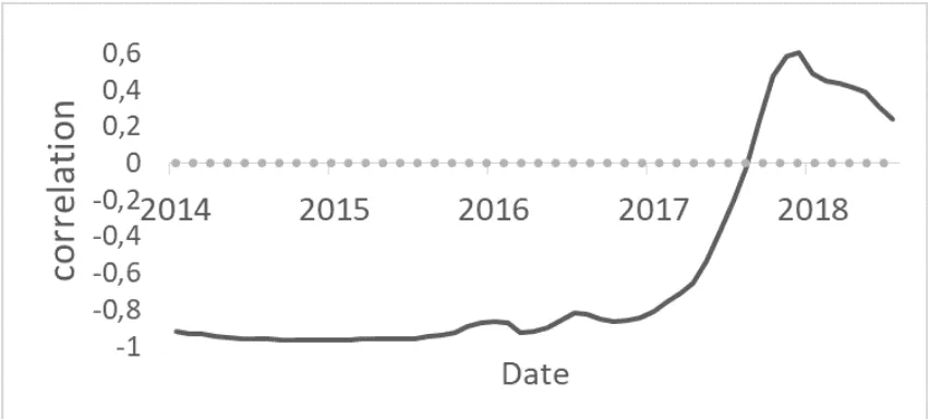
uncertainty. Before 2017 year, oil prices had almost one-to-one correlation with exchange rate USD/RUB.
Fig. 1 illustrates the moving average correlation between oil prices and exchange rate USD/RUB.
Note: The monthly moving average correlation is calculated in the following way. For each month the 12 months before and 12 months after are considered. For these 25 obser-vations the correlation coefficient between Brent oil price and exchange rate USD/RUB is calculated.
Figure 1. Two-year moving average correlation between oil prices and exchange rate
USD/RUB
Negative oil price shocks resulted in rubble weakening. The latter leads to inflation increase due to
exchange rate path-through effect. Thus, monitoring oil prices could allow central bank to timely react
to future changes in inflation. Starting from 2014 year, some foreign countries introduced a range of
sanctions on Russia. One of the effects of sanctions is the rubble weakening. Russia is a small open
economy; exchange rate fluctuations have a significant effect on internal inflation. Bank of Russia could
possible react with policy rate hike in response to exchange rate weakening. By doing so Bank of Russia
could smooth future exchange rate pass-through effect in inflation. A set of restrictions on endogenous
monetary policy is the following. Central bank hikes policy rate in response to inflation increase, exchange
rate weakening. Central bank does not respond to changes in output or unemployment. The one period
impulse response functions restrictions are similar to monetary policy rule I.
Monetary policy rule III:
To check whether the central bank reacts to output fluctuations, I implement other monetary policy
rule. A set of restrictions on endogenous monetary policy is the following. Central bank hikes policy
rate in response to inflation increase, output increase, exchange rate weakening. Central bank does not
to monetary policy rule I. If impulse response functions of inflation to monetary policy shocks in rules II
and III are identical, then adding output response in feedback rule is excessive. The one period impulse
response functions restrictions are similar to monetary policy rule I.
Second step, I re-run the series in a way to clean the data from monetary policy shocks. Define ˆ𝑌t
as counterfactual series which are subject to all the shocks except for the monetary policy shocks. The
model is identified via (Uhlig, 2004) approach to explain a maximum forecast error variance of policy rate,
cleaned from monetary policy shocks, at five year horizon.
ˆ
𝑌t =𝐶0+𝐶1𝑌tˆ−1+...+𝐶k𝑌tˆ−k+𝐷0𝑢t (2)
Where 𝐶k is the 𝑛×𝑛 matrix of parameters given 𝑘 ∈[0,1, . . . , 𝑘+ 1, .., 𝑝], 𝑝 is a maximum lag order
of VAR in canonical form identical to the first step. 𝐷0 is the 𝑛×𝑛 matrix of structural shocks,𝑢t is the
vector of𝑛×1 structural shocks at period 𝑡.
III. Data
The dataset contains monthly Russian data on oil prices (Oil), interbank interest rate (MIACR) from 2
to 7 days, consumer price index (CPI), unemployment (U), exchange rate USD/RUB (ExR), two economic
activity series: index of industrial production (IPI) and index of output of key branches (IBI) from January
2014 to July 2019. The source of Brent oil prices is FINAM. The source of CPI, U, IPI, IBI is Federal
State Statistic Service. The source of exchange rate and MIACR is Bank of Russia. I calculate monthly
growth rates for oil prices, exchange rate, CPI, IPI, IBI and keep unemployment and MIACR at levels. The
number of variables is identical to (J.E. Arias et al., 2019) except for total reserves, nonborrowed reserves.
I exclude the latter variables because Bank of Russia never targeted them during the period of analysis.
Except for the exchange rate and MIACR, all the series are seasonally adjusted with X13-ARIMA-SEAT.
IV. Results
In this section, I first choose the best monetary policy rule. Then, I cover benefits and drawbacks of
Implicit monetary policy rule
To choose the implicit monetary policy rule, I rely on analysis of impulse response functions and policy
feedback rule. Standalone, it is not sufficient to compare either impulse response functions or policy
feedback across different monetary policy rules. Policy feedback rule is defined by coefficients in VAR
model. Impulse response functions are additionally determined by matrix of structural shocks. Both
coefficients and structural matrix differ from monetary policy rule one to three. Going from monetary
policy rule one to three, I impose additional information on central bank behaviour, being the third rule
with the most number of restrictions. If augmentation of information keeps the reaction of inflation to
monetary shocks and feedback rule the same, then such constrains are excessive. To assess the uncertainty
around the estimates I perform bootstrap procedure.
Matrix of structural of shocks is not fully identified in (J.E. Arias et al., 2019) procedure. Therefore,
I choose a number of rotation matrices1
to characterize uncertainty around the identification. Further,
I perform bootstrap procedure2
to describe uncertainty around the path of matrices of structural shocks
estimates. I calculate all further confidence intervals for impulse response functions, policy feedback rules,
forecast error variances decompositions, structural shocks and counterfactual simulations via bootstrap.
To discuss monetary policy rules, I include unemployment (U), interbank interest rate (MIACR) from
2 to 7 days, consumer price index (CPI), exchange rate USD/RUB (ExR), index of output of key branches
(IBI). I exclude oil prices from the analysis subject to several reasons. First, oil prices mainly characterize
the state of the foreign markets. Exchange rate includes this information. Prior to 2017 year, the dynamics
of oil prices and exchange rates was almost one-to-one. Secondly, the period of analysis is limited; I prefer
to shrink the number of included variables to five to decrease uncertainty around coefficients estimates.
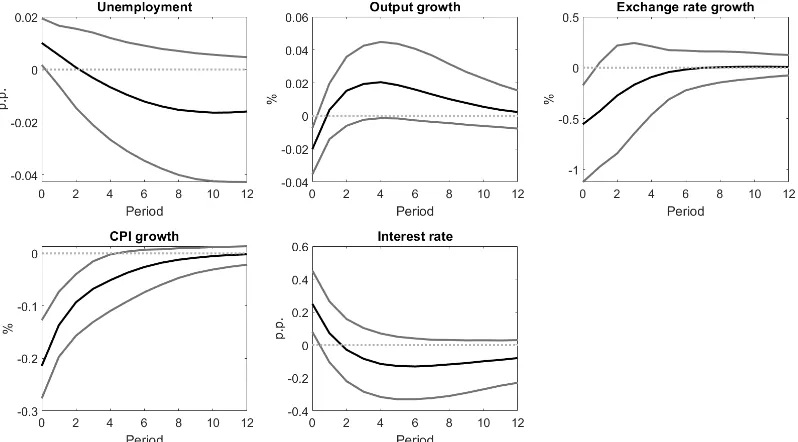
In (fig. 2) I draw the response of macroeconomic variables to unit monetary policy shock under the first
monetary policy rule.
The results show that unexpected interest rate hike leads to the decline of economic activity. CPI
becomes lower, output declines, unemployment increases. There is no price or output puzzles. The rubble
becomes stronger because interest rate hike makes the economy more attractive for foreign investors. They
can get higher returns for a rubble of investments, thus foreign investors increase demand for rubble and
its price. The results are significant for exchange rate, output and unemployment for one month.
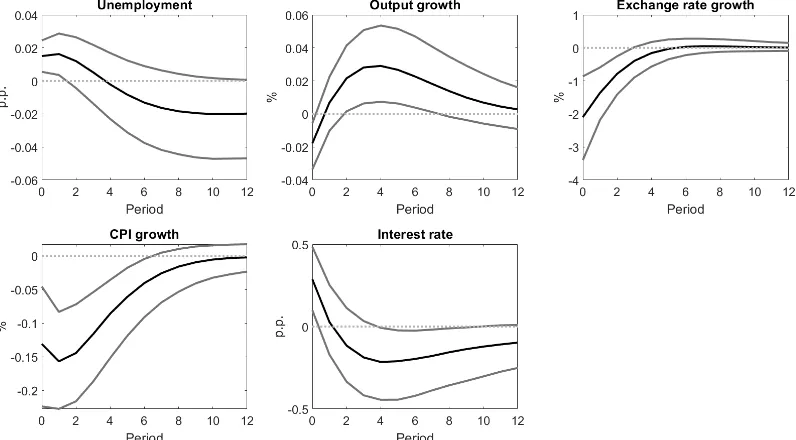
In (fig. 3), I augment restrictions by imposing the reaction of a central bank to an exchange rate in
1Number of rotation matrices is equal to 100
2Number of bootstrap samples is equal to 1000. Total number of simulating paths is less or equal than 100 000. In
practice, the number of draws cannot be exactly equal to 100 000. I reject all the draws that do not satisfy monetary policy
Note: The black line is median point estimate of the draws that satisfy monetary pol-icy rule I. The grey lines are one-standard deviation confidence intervals: 16% and 84% percentiles. The period is equal to 1 month.
Figure 2. Impulse response functions to unit monetary policy shock under monetary
policy rule I
policy feedback rule. The response of inflation has changed from parabolic to hump-shaped. The effect
of shock has distributed more smooth along the periods. Moreover, the period of inflation response has
increased from four to seven months. Exchange rate response has also increased its significant path to four
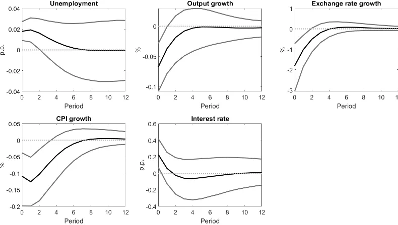
months. Further, in (fig. 4) the restrictions are augmented by the endogenous response of a central bank
to changes in output.
Responses of macroeconomic variables to identical monetary policy shocks are almost the same (at
90% level) under monetary policy rules II and III. Thus, I draw a conclusion that monetary policy rule II
is sufficient to obtain canonical impulse responses1
. I further investigate policy feedback under different
monetary policy rules. Equation (1) implies the following feedback rule:
𝑀 𝐼𝐴𝐶𝑅t=𝛽0+𝛽y𝐼𝑃 𝐼t+𝛽π𝐶𝑃 𝐼t+𝛽er𝐸𝑋𝑅t+𝛽u𝑈t+
p
∑︁
k=1
[𝐿k(𝛽y𝐼𝑃 𝐼k+𝛽π𝐶𝑃 𝐼k+𝛽er𝐸𝑋𝑅k+𝛽u𝑈k)]+ N
∑︁
i=1
𝛼0i𝜖it
(3)
Where 𝛽j are feedback coefficients of our interest𝑗 = 1, . . . , 𝑁 + 1, 𝑁 is a number of variables, 𝐿k is a
1The results for impulse response functions in case of the absence of sign restrictions on exchange rate and output are
similar. Monetary policy rule II without these restrictions also produces canonical impulse responses. For the sake of space,
Note: The black line is median point estimate of the draws that satisfy monetary pol-icy rule I. The grey lines are one-standard deviation confidence intervals: 16% and 84% percentiles. The period is equal to 1 month.
Figure 3. Impulse response functions to unit monetary policy shock under monetary
policy rule II
lag operator of order𝑘, the maximum lag order is equal to one,𝛼0
i𝜖𝑖𝑡is a multiple of the first raw structural
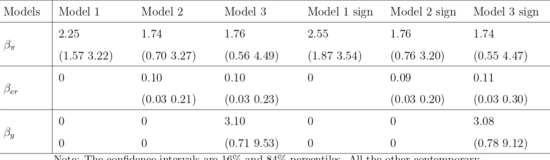
shocks coefficients by structural shocks. I summarize the results in (tab. 1):
Table 1 implies that for the second and third monetary policy rules under or without sign restrictions
endogenous reaction of a central bank is identical. However, one can still observe differences for the first
feedback rule. In general, the 1 percentage point of inflation increase should result in 1.75 percentage
points hike of the interest rate. The 10% rubble weakening should result in 1 percentage points hike of
the interest rate. The 1% of additional economic growth should result in 1 percentage points hike of the
interest rate. Together with impulse response functions, feedback rules suggest that monetary policy rule
II is sufficient, while the third rule does not help in estimation of IRFs and policy rules. All further results
are presented for monetary policy rule II.
Monetary policy shocks itself are of the interest in this paper. Shocks allow describing the episodes
of monetary policy decisions from the expectation perspective. Bloomberg and Reuters regularly survey
analytics before and after decisions of the Bank of Russia Board of Governance. Thus, central bankers
can understand whether their changes of policy rates are in line with the projections of the analytics.
Such surveys provide evidence on the efficacy of forward guidance policy. Nevertheless, analytics are only a
Note: The black line is median point estimate of the draws that satisfy monetary pol-icy rule I. The grey lines are one-standard deviation confidence intervals: 16% and 84% percentiles. The period is equal to 1 month.
Figure 4. Impulse response functions to unit monetary policy shock under monetary
policy rule III
estimate monetary policy shocks for overall economy; hence, shocks better reflect whether the expectations
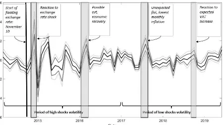
of policy rate changes correspond to the actual hikes, cuts or flats. Fig. 5 describes various episodes of
monetary policy shocks on the example of four statistically significant shocks.
Bank of Russia suspended exchange rate market operations on November 10. I correspond this date to
the beginning of the floating exchange rate regime. In two months rubble exchange rate plummeted almost
two times due to an oil price shock. Bank of Russia reacted to inflation shock and raised the policy rate
up to 17%. Such an increase was an unexpected hike to economic agents. At that time, central bank just
started the inflation targeting and the communication could not be effective. The end of 2014-year shock
is the highest shock with the point estimate to be 2.4, and the upper 68% boundary up to 4.0 percentage
points. March 2016 reflect and summer 2017 are the episodes which shed light on the concept of monetary
policy shocks. Though, in these periods the policy rate was flat indeed economy experienced shocks.
According to Bloomberg, 21 out of 39 analytics were expecting policy rate cut on June 2017. The Board
of Governance decision to keep the policy rate flat was unexpected to analytics, and hence, the decision can
be characterized as a shock. The peak shock in summer 2017 is 1.5 percentage points. Analytics found the
economy recovery supported by the lowest monthly seasonally adjusted inflation on August 2017; they were
Table 1. Monetary policy feedback rule contemporary coefficients
Models Model 1 Model 2 Model 3 Model 1 sign Model 2 sign Model 3 sign
𝛽π
2.25 1.74 1.76 2.55 1.76 1.74
(1.57 3.22) (0.70 3.27) (0.56 4.49) (1.87 3.54) (0.76 3.20) (0.55 4.47)
𝛽er 0 0.10 0.10 0 0.09 0.11
(0.03 0.21) (0.03 0.23) (0.03 0.20) (0.03 0.30)
𝛽y
0 0 3.10 0 0 3.08
0 0 (0.71 9.53) 0 0 (0.78 9.12)
Note: The confidence intervals are 16% and 84% percentiles. All the other contemporary coefficients are equal to zero. “MP” stands for the abbreviation of monetary policy rule, the mark “sign” means that I additionally impose sign restrictions on exchange rate and output.
data all out of 16 people, were expecting policy rate flat. Bank of Russia hiked policy rate to prevent future
consequences of VAT pass-through on inflation. This episode is an example of unexpected hike. Overall,
the standard deviation of monetary shocks has decreased from 1.08 during the 2014 and 2017 years to 0.38
afterwards. The volatility dynamics shrinkage could be attributed to the rising efficacy of forward guidance
and budget rule.
Benefits and drawbacks of (J.E. Arias et al., 2019) method on the Russian
example
The previous results suggest that there is an absence of output and price puzzles, the impact of monetary
shocks on inflation and other variables is statistically significant. My results are different from those
obtained for Russian economy earlier. The paper (Borzyh O. A., 2016) studies the transmission of monetary
shocks to volume of credits. The author exploits recursive identification and obtains that the contractionary
effect of monetary policy can be observed only on some subsamples. Another paper (Pestova, A. A. et al.
2019) supports that contractionary monetary policy does not lead to the inflation slowdown by applying
factor analysis with sign restrictions. The other paper (Shestakov, D. E., 2017) finds evidence on the
absence of cost channel in Russian economy. All these papers apply either recursive identification or sign
restrictions on impulse response functions.
The problem with such identifications is that they allow a central bank to react in a policy irrelevant
way. For instance, if there is an output slowdown, than central bankers can hike interest rate. (J.E. Arias
Note: The black line is median point estimate of the draws that satisfy monetary policy rule II. The grey lines are one-standard deviation confidence intervals: 16% and 84% percentiles. The dotted grey lines are two-standard deviation confidence intervals: 5% and 95% percentiles.
Figure 5. Monetary policy shocks under monetary policy rule II
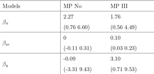
To provide evidence that such restrictions are meaningful, I have estimated the feedback rule under sign
restrictions on impulse response function and without feedback rule restrictions (tab. 2). The absence of
feedback rule restrictions results to a nonzero probability hike of policy rate in response to exchange rate
strengthening or output declining.
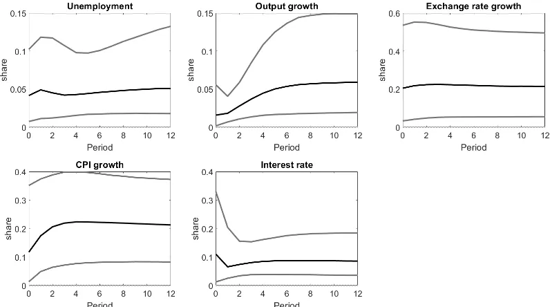
To further investigate the appropriateness of identification applied in this paper, I estimate forecast
error variance decompositions (fig. 6).
Monetary policy shocks explain 10% of interest rate dynamics and 20% of CPI growth. Though the
shares of explanation are meaningful, they are small. I cannot compare forecast error variance
decomposi-tions with (J.E. Arias et al., 2019) paper because they do not provide these results1
. The question is what
does explain the rest of inflation and policy rate?
Natural interest rate results
Natural interest rate could shed light on small forecast error variance decompositions under monetary
policy shocks. I identify natural interest rate shocks to the series cleaned from monetary policy shocks
1Nevertheless, one can reproduce the results of (J.E. Arias et al., 2019) and get that monetary policy shocks explain less
Table 2. Unrestrictive monetary policy feedback rule
Models MP No MP III
𝛽π
2.27 1.76
(0.76 6.60) (0.56 4.49)
𝛽er 0 0.10
(-0.11 0.31) (0.03 0.23)
𝛽y
-0.09 3.10
(-3.31 9.43) (0.71 9.53)
Note: The confidence intervals are 16% and 84% percentiles. All the other contemporary coefficients are equal to zero. “MP” stands for the abbreviation of monetary policy rule, the mark “no” means that I impose sign restrictions on impulse response function and do not impose feedback rule restrictions.
via (Uhlig, H.,2004) approach. From the rest of the shocks I choose the linear combination of those that
best explain the cleaned policy rate at five-year horizon. Five-year period is sufficient to decimate the
effect of temporary nominal shocks. Output itself is driven itself by demographic trends, total factor
productivity shocks, total factor productivity shocks, budget policy shocks. Hence, these long-term factors
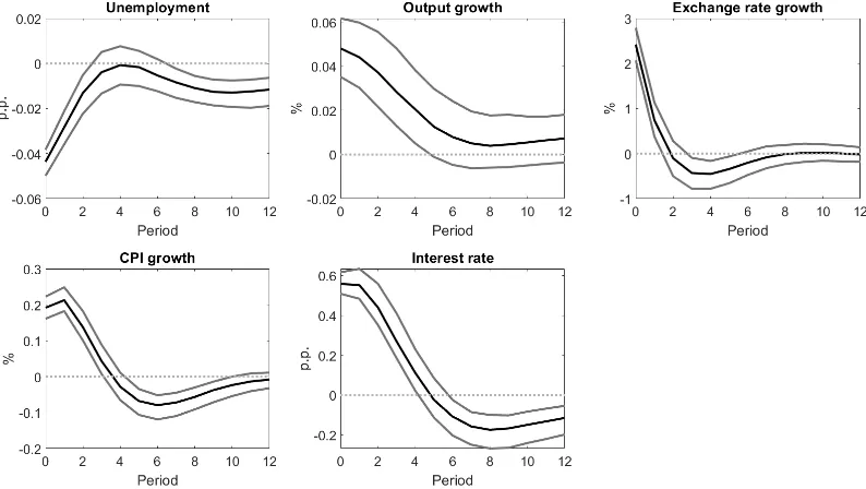
could explain natural interest rate shocks. The (fig. 7) depicts the impact of unit natural interest rate
shock on macroeconomic variables.
The results of natural interest identification suggest that natural interest rate increase lead to CPI
and output increase. Suppose that natural interest rate is lower than the policy rate. Hence, there is a
contractionary effect of monetary policy of economy. The economy is hit by a positive natural interest
shock. The difference between the natural interest rate and policy rate shrinks namely the natural interest
rate goes up more than policy rate. Thus, the contractionary effect of monetary policy declines. There
is a stimulating effect of a positive natural interest rate shock on inflation and output. Natural interest
rate shocks explain about 60% of consumer prices variation and around 30% of output (Appendix A).
The variance of policy rate, inflation and output that not explained by monetary policy shocks is mostly
explained by natural interest shocks. Monetary policy shocks and natural interest rate shocks altogether
explain up to 90% of variation in inflation. These two types of shocks are sufficient to describe the stance
of monetary policy.
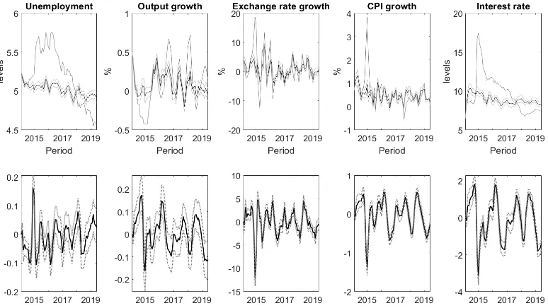
I suppose that the only drivers of changes in natural interest rate are natural interest rate shocks. I
perform counterfactual simulations (fig. 8) where are keep only natural interest rate shocks. The (fig.
8) illustrates that natural interest rate (the upper-right graph) is declining from 13% in 2015 year to 6%
Note: The black line is median point estimate of the draws that satisfy monetary policy rule II. The grey lines are one-standard deviation confidence intervals: 16% and 84% percentiles. The period is equal to 1 month.
Figure 6. Forecast error variance decompositions of monetary policy shock under
monetary policy rule II
variable to the index of production function then natural rate becomes less volatile (Appendix B). Overall,
[image:16.612.114.512.37.259.2]Note: The black line is median point estimate of the draws that satisfy monetary policy rule II, which essentially means that all the series were cleaned from the monetary policy shocks under monetary policy rule II. The grey lines are one-standard deviation confidence intervals: 16% and 84% percentiles. The period is equal to 1 month.
Figure 7. Impulse response functions to unit natural interest rate shock
Conclusion
This paper propose a procedure of identification of monetary policy and natural rate shocks the
domi-nating drivers of monetary policy stance. To disentangle natural rate shocks from monetary policy shocks,
I perform a two-stage procedure. Firstly, I estimate monetary policy shocks. Secondly, I clean out the
series from the impact of monetary policy shocks and explain the rest of policy rate variance by the natural
interest shocks1
.
To identify monetary policy shocks, I exploit (J.E. Arias et al., 2019) procedure, which allows to get
canonical impulse response functions. Further, I interpret monetary policy shocks during the period of
Bank of Russia inflation targeting. Overall, shocks resemble the expectations of professional analytics.
The novel identification procedure of natural interest rate shocks allows to quantitatively estimate the
impact on natural interest rate shocks on macroeconomic variables, to characterize the stance of monetary
policy. The natural rate estimates support the global tendency of declining rates.
1One could answer the question whether is it possible to firstly identify natural interest rate shocks and secondly detect
monetary policy shocks. In that case long-term natural interest shocks will be distorted by short-term monetary policy shocks.
To provide some evidence on this, in Appendix C I estimate natural interest rate shocks without the first stage. The results
are poor: the response of output is insignificant, the response of inflation lasts for only one month and the unemployment
Note: The black line is the median estimate of the series driven by only natural interest rate shocks. The light grey lines are one-standard deviation confidence intervals: 16% and 84% percentiles. The grey lines are actual series.
Figure 8. Counterfactual simulations of the series driven by only natural interest rate
shocks
The further investigation could include the analysis of factors that resulted in natural interest rate
shocks. One could also develop a model whether the monetary policy and natural interest shocks will
be determined simultaneously. The limitation of the current approach is that there is double uncertainty
coming from cleaning of monetary policy shocks and estimates of natural interest rate shocks. In current
paper, I neglect the first uncertainty and work with the median values of series cleaned out from monetary
References
[1] Amato, J. D. (2005). The role of the natural rate of interest in monetary policy. CESifo Economic
Studies, 51(4), 729-755.
[2] Arias, J. E., Caldara, D., & Rubio-Ramirez, J. F. (2019). The systematic component of monetary
policy in SVARs: An agnostic identification procedure. Journal of Monetary Economics, 101, 1-13.
[3] Barsky, R. B., & Sims, E. R. (2011). News shocks and business cycles. Journal of monetary Economics,
58(3), 273-289.
[4] Benati, Luca (2019) “A new approach to estimating the natural rate of interest.” Mimeo, University
of Bern.
[5] Christiano, L. J., Eichenbaum, M., & Evans, C. L. (1999). Monetary policy shocks: What have we
learned and to what end? Handbook of macroeconomics, 1, 65-148.
[6] Holston, K., Laubach, T., & Williams, J. C. (2017). Measuring the natural rate of interest:
Interna-tional trends and determinants. Journal of InternaInterna-tional Economics, 108, S59-S75.
[7] Laubach, T., & Williams, J. C. (2003). Measuring the natural rate of interest. Review of Economics
and Statistics, 85(4), 1063-1070.
[8] Laubach, T., & Williams, J. C. (2016). Measuring the natural rate of interest redux. Business
Eco-nomics, 51(2), 57-67.
[9] Orphanides, A., & Williams, J. C. (2002). Robust monetary policy rules with unknown natural rates.
Brookings Papers on Economic Activity, 2002(2), 63-145.
[10] Ramey, V. A. (2016). Macroeconomic shocks and their propagation. In Handbook of macroeconomics
(Vol. 2, pp. 71-162). Elsevier.
[11] Ramsey, F. P. (1928). A mathematical theory of saving. The economic journal, 38(152), 543-559.
[12] Uhlig, H. (2004). Do technology shocks lead to a fall in total hours worked?. Journal of the European
Economic Association, 2(2-3), 361-371.
[13] Walsh, C. (1998). Monetary Theory and Policy The MIT Press. Cambridge MA.
[14] Borzyh, O. A. (2016). Kanal bankovskogo kreditovaniya v Rossii: ocenka s pomoshch’yu TVP-FAVAR
[15] Pestova, A. A., Mamonov, M. E., & Rostova, N. A. (2019). Shoki Procentnoj Politiki Banka Rossii
i Ocenka Ih Makroekonomicheskih Effektov. Ekonomicheskaya politika, 14(4) (in Russian). Quarterly
Journal of Economics, 105(2), pp. 255–83.
[16] Shestakov, D. E. (2017). Kanal izderzhek denezhno-kreditnoj transmissii v rossijskoj ekonomike. Den’gi