Dependency Parser for Sanskrit Verses

Dependency Parser for Sanskrit Verses

Amba Kulkarni, Sanal Vikram and Sriram K Department of Sanskrit Studies

University of Hyderabad

[email protected],[email protected],[email protected]

Abstract

Sentence parser is an essential component in the mechanical analysis of natural language texts. Building a parser for Sanskrit text is a challenging task because of its free word order and the dominance of verse style in Sanskrit literature in comparison to prose style. In this paper, we describe our efforts to build a parser which parses both prose as well as verse texts. It employs an Edge-Centric Binary Join method using various constraints following traditional rules of verbal cognition. We also propose a Daṇḍa-anvaya-janaka which converts the parsed verse form to its canonical prose order.

1 Introduction

Parsing natural language sentences automatically to reveal the underlying semantics has at-tracted many researchers to this field in the past two decades. The parse of a sentence is useful for several applications ranging from machine translation, information retrieval to question an-swering. Parsing sentences with fixed word order is comparatively easier than parsing texts that show some flexibility in the word order. We come across such flexibility in poetry. The syntax and semantics of poems have been an area of serious studies. Delmonte (2018) studies the syntax and semantics of Italian poetry. He observes that the best parsers for Italian based on statistical probabilistic information fail to parse poetic structures while the rule based system performs well. Lee and Kong (2012) have noticed the importance of treebank for poems in order to use the statistical or machine learning models, and have developed a dependency treebank for Classical Chinese poems. The Stanford Dependency relations were extended in order to account for certain poetic constructs in Chinese.

Krishna et al. (2019) proposed a model, called kāvya guru, for the conversion of Sanskrit sentences in verse to prose form, which considers the task of conversion as a linearisation prob-lem. It first uses—Dynamic Meta Embeddings (DME)—for training, where it forms a single meta embedding from multiple pretrained word embeddings of a given token. Then it uses a linearisation model—Self-Attention Based Word Ordering (SAWO)—which generates multiple permutations of words, which are then sent to a seq2seq model that produces the required prose order form. They compared the performance of their system with an LSTM based Linearisation Model, and seq2seq model with Beam Search Optimisation, and their system performs the best with a BLEU score of 55.26.

In this paper we describe a parser for Sanskrit that can parse both verse and prose. In the next section we describe the basic architecture of our parser that extracts a tree from a graph satisfying some local and global constraints. In the third section we provide the algorithm for constraint solver and illustrate it with an example. Next two sections describe an application of this parser to get the prose order (also termed daṇḍa-anvaya) of any verse. We conclude with the discussion on the performance of the parser stating its limitations and the areas where it needs further improvement.

2 Design of a Parser

We find two main approaches towards the design of a dependency-based parser. They are Gram-mar based and Data driven. The Link parser (Sleator and Temperley, 1993) based on Link grammar formalism and the Minipar (Lin, 1998) based on Chomsky’s Minimalism are among the grammar based dependency parsers. Data-driven dependency parsers are the state-of-art parsers. They use supervised machine learning algorithms to train the machine on annotated corpus. These parsers need manually annotated corpus, called tree banks, for training. Among these parsers, we come across two dominating approaches. They are graph-based dependency parsing and transition-based dependency parsing. The graph-based approach creates a parser model that assigns scores to all possible dependency graphs and then uses maximum span-ning tree methods from Graph theory for getting the highest-scoring dependency graph. The transition-based approach scores transitions between parser states based on the parse history and then follows a greedy approach and produces a single parse corresponding to the highest-scoring transition sequence that derives a complete dependency graph.

Most of the natural language parsers call a part of speech(POS) tagger and a chunker before invoking a parser. These two modules reduce the ambiguity due to multiple morphological analyses. A POS tagger selects the best part of speech in the context, and a chunker groups all the auxiliary verbs with the main verbs, the post-positions with the noun, and multi-word expressions as one chunk. The head of such chunks is marked which relates to other words or heads of other chunks in a sentence. The POS taggers and chunkers ease the task of a parser, by reducing the ambiguities at the morphological level. However the disadvantage of calling these modules before a parser is that the errors may get cascaded.

Our parser differs from the state-of-the-art parsers in three ways. First, in the absence of any annotated corpus, we follow the grammar based approach. Secondly, our parser is invoked right after the morphological analyser. The main reason behind this decision was the following. Indian literature on verbal import was found to be useful from parsing point of view since it has discussions on various factors that are instrumental in the process of verbal cognition. Our main goal is to build a parser modeling the theories of śābdabodha. When we looked at various Indian literature related to the theories of verbal cognition, there was no discussion on any kind of POS tagger or chunker. Moreover, use of chunker also presupposes that dependencies relate the whole chunk and do not involve a sub-part of it. But in Sanskrit we come across instances of compounds termed as asamartha-samāsa (Joshi, 1968; Gillon, 1993) where the dependencies relate to the sub-part of a compound which need not necessarily be a head. Use of a chunker module before calling a parser would fail to parse such constructs. Finally, the state-of-art parsers typically produce a single parse. We decided to produce all possible parses. This is to ensure that we do not miss out the correct parse. The onus of choosing the correct parse, from among the parses produced, is on the reader.

The challenge before us was to handle the free word order in Sanskrit both in prose as well as in verse. The basic algorithm we followed for parsing is given below.

1. Define one node each corresponding to each morphological analysis of every word in a sentence.

mu-tually incongruous (yogyatā).

3. Define constraints, both local on each node as well as global on the graph as a whole. One of these constraints corresponds to sannidhi (proximity).

4. Extract all possible trees from this graph that satisfy both local and global constraints. Pro-duce all possible solutions to ensure that in case of sentences with multiple interpretations,1 machine does not miss any interpretation.

5. Produce the most probable solution as the first solution by defining an appropriate cost function. The cost C associated with a solution tree is defined asC =∑_ede×rk, where e is an edge from a wordwj to a wordwi with labelk,de=|j−i|,rk is the rank2 of the role with label k.

Then the problem of parsing a sentence may be modeled as the task of finding a sub-graphT of Gsuch thatT is a Directed Tree.

To start with, in order to get familiarity with the kind of problems due to ambiguity, we designed a parser (Kulkarni et al., 2010) that handles a text in formally defined canonical prose order. This parser was implemented as a constraint solver. This parser was found to be very inefficient due to the use of matrix data structure which resulted in sparse matrices for long sentences or sentences with heavily ambiguous words at morphological level, affecting the efficiency. This algorithm was later improved by using vertex-centric traversal using dynamic programming (Kulkarni, 2013). The major disadvantage of this method is, being node-centric traversal, if the initial words have several incoming arrows, then the number of partial solutions in the beginning are many and as one traverses various paths, the possibilities grow exponentially. It also checks the compatibility of each new edge with all the edges on the path explored so far. This leads to some redundancy, since if a node falls on more than one path, it would be visited more than once, and during each such visit all the incoming edges are checked for compatibility with all other edges on the path traversed so far. In the worst case scenario the incompatibility between the nodes would be noticed only at the final node.

Both these algorithms were designed for sentences that have a default SOV order. Now we present below an algorithm that is designed to handle both prose as well as verse order. This algorithm also overcomes the disadvantages of the earlier algorithm viz. the redundancy in compatibility checking. It has been observed that the arguments having mutual expectancy (utthita ākāṅkṣā), such as the core arguments of a predicate, follow weak non-projectivity while the arguments having unilateral expectancy (utthāpya ākāṅkṣā) are exceptions to this rule (Kulkarni et al., 2015). We use these constraints to extract a tree from the graph.

3 Edge-centric Binary Join

We modify the previous algorithm at three levels.

1. Any edge that is a part of the solution should be compatible with remaining n−2 edges in the solution tree, wherenis the number of words in the sentence. This is to ensure that the solution hasn−1 edges. Hence, all those edges that are not compatible with at least n−2other edges are thrown away.

2. We define the compatibility of two sets of edges as a simple operation of set intersection. 3. We build the solutions recursively starting with the individual words bottom-up, each time

joining two sets of compatible edges. In n−1 joins we get all possible directed acyclic graphs (DAG), where nis the number of words in a sentence. Join operation is defined as a set union. These DAGs are Directed Trees, since each DAG involvesn nodes withn−1

edges with all the words connected. This algorithm is edge-centric.

Before giving the detailed algorithm, we define a few terms. 1. Local constraints:

(a) A morpheme corresponding to a suffix marks only one relation. That is, a node can have one and only one incoming edge. (b) Each kāraka relation is marked by a single morpheme.

There cannot be more than one outgoing edge with the same label from the same node, if the relation corresponds to a kāraka relation,3 i.e. there cannot be two words satisfying the same kāraka role of the same verb.

(c) A morpheme does not mark a relation to itself.

A word cannot satisfy its own expectancy, i.e. a word cannot be linked to itself. (d) There can be only one valid analysis of every word per solution. Since a word has one

node corresponding to each morphological analysis it has, there are further restrictions as below.

i. If a word has both an incoming edge as well as an outgoing edge, they should be through the same node.

ii. If there is more than one outgoing edge for a word, then all of them should be through the same node.

iii. A viśeṣaṇa cannot have a viśeṣaṇa.4

These conditions ensure that only one morphological analysis is chosen per word. 2. Global Constraints:

(a) Sannidhi: There are no crossing of edges.

If all the nodes are plotted in a straight line, then the edges connecting them (drawn on the upper side of the line) should not intersect each other. Adjectival relation and the relation due to genitive suffix are exceptions to this rule.

(b) Certain relations always occur in pairs. For example, a kartṛsamānādhikaraṇa (a pred-icative adjective, literally having same locus as that of kartṛ) assumes that there is a relation of kartṛ already established.

3. Compatible edge:

An edge e1 is said to be compatible with another edgee2 if they satisfy local constraints,

and we setCompatible(e1, e2) = 1.

4. Compatible set of edges:

Let R be a set with edges {r1,r2,…,rn}, and S be a set with edges {s1,s2,…,sm}. S is

compatible with R iff_{∀i ∀j} Compatible(si, rj) = 1. 5. Joinable sets:

LetR1 andR2 be two sets of edges. LetS1 andS2 be the sets of edges that are compatible

withR1 and R2 respectively. R1 and R2 are joinable provided R1 ⊆S2 and R2 ⊆S1. For

such joinable sets, the edges compatible withR1 ∪R2 are defined as (S1 ∩S2) - (R1 ∪R2).

Now we give the detailed algorithm. 1. Let there beN edges.

2. For each edge, list down all other edges it is locally compatible with. 3. Construct all possible DAGs, by calling ConstructDags0 N,

where ConstructDags is defined as ConstructDags initial final =

if (final - initial > 0) then

dags = RemoveSmallDags size (JoinDags dag1 dag2) where

size = final - initial -1

dag1 = ConstructDags init mid, and

3_{adhikaraṇa is treated as an exception since one can have more than one adhikaraṇa as in—}

Skt: rāmaḥ adya pañca vādane gṛham agacchat

Eng: Today Rama came home at five o’clock.

dag2 = ConstructDags (mid+1) final, where mid = (initial + final) / 2 else

dags = GetInitialDags init,

which returns as many initial DAGs as there are incoming arrows at the node with index init. Each such initial DAG contains a single incoming arrow. RemoveSmallDags N dags

removes all the DAGs, from dags that have less thanN edges. JoinDagsD1 D2

joins two dagsD1 and D2, if they are joinable sets, and for

the combined dagD, compute the edges compatible withD.

4. Remove all those solutions that do not satisfy the global compatibility condition.

5. For each globally compatible solution, compute the costCdefined asC=∑_ede×rk, where eis an edge from a word wj to a word wi with label k,de=|j−i|,rk is the rank5 of the role with labelk. and then prioritise the solutions based on this cost.

3.1 An Example

We illustrate the algorithm with the following simple sentence.

San: gacchati rāmaḥ vanam. (1)

gloss: Goes Ram forest{acc.}. Eng: Ram goes to the forest.

In this sentence, each of the two words rāmaḥ (Ram) and vanam (forest) has two possible analyses, and the wordgacchati (goes) has three possible analyses as shown below.

0. rāmaḥ = rāma {masc.} {sg.} {nom.} 1. rāmaḥ = rā {pr.} {1p} {pl.}

2. vanam = vana {neu.} {sg.} {nom.} 3. vanam = vana {neu.} {sg.} {acc.} 4. gacchati = gam {pr.} {3p.} {sg.}

5. gacchati = gam {pr. part.} {masc.} {sg.} {loc.} 6. gacchati = gam {pr. part.} {neu.} {sg.} {loc.}

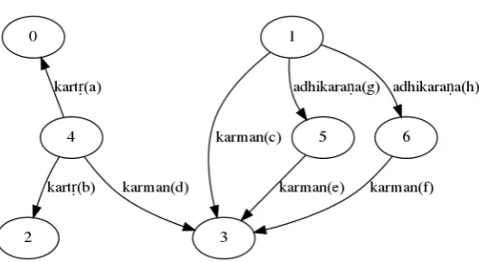
Figure 1: All possible relations for sentence 1

All possible relations are shown in Figure 1 and their compatible relations in Table 1.

Edge From To Relation Name Compatible

ID (j) (i) (r) Edges

a 4 0 kartṛ d

b 4 2 kartṛ

-c 1 3 karman g,h

d 4 3 karman a

e 5 3 karman g

f 6 3 karman h

g 1 5 adhikaraṇa c,e

h 1 6 adhikaraṇa c,f

Table 1: All possible edges and their compatible edges

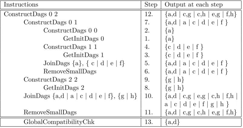
Instructions Step Output at each step

ConstructDags 0 2 12. {a,d | c,g | c,h | e,g | f,h} ConstructDags 0 1 7. {a,d | a | c | d | e | f }

ConstructDags 0 0 2. {a}

GetInitDags 0 1. {a}

ConstructDags 1 1 4. {c | d | e | f } GetInitDags 1 3. {c | d | e | f }

JoinDags {a}, { c | d | e | f} 5. {a,d | a | c | d | e | f } RemoveSmallDags 6. {a,d | a | c | d | e | f }

ConstructDags 2 2 9. {g | h}

GetInitDags 2 8. {g | h}

JoinDags {a,d | a | c | d | e | f}, {g | h} 10. {a,d | c,g | e,g | c,h | f,h | a | c | d | e | f | g | h } RemoveSmallDags 11. {a,d | c,g | c,h | e,g | f,h}

GlobalCompatibilityChk 13. {a,d}

Table 2: Trace of algorithm on sentence 1

First we filter out edge b, since it is not compatible with any of other edges. We retain all other edges as they are compatible with at least 1 (=n−2) other edge. Next we start building the solutions recursively. We start with the incoming edges of the first word. There is only one incoming edge, marked as a. This forms our first set of edges R1. The set of compatible edges

withR1, denoted byS1 has only one edged. For the second word there are four incoming edges,

marked asc,d,e, andf. Each of these starts a new partial solution. We call themR2,R3,R4,

and R5. For each of these edges, the compatible edges are shown in Table 1. We call them S2,

S3,S4, andS5 respectively. Now we check which of these partial solutions are joinable withR1.

We notice that only R3 is joinable with R1. Joining these two partial solution sets, results in

{a,d}. The set of edges compatible with this partial solution is given by (S_{1 ∩} S3) - (R1 ∪R3)

=ϕ. We carry earlier partial solutions viz. R2,R3,R4, and R5, as well, being potential partial

solutions, since each of them has one edge, and we still have one more word to visit. Now we get the edges of the third word, and join them with the current partial solutions. Corresponding to the third word, we have gand h as two incoming edges. Checking compatibility with all the partial solutions in the previous stage, we get five possible solutions as shown in Figure 2. In Table 2, we show the invocation of the algorithm for this sentence. The result shows the step number followed by the list of possible relations at that step. In this trace, we have not shown the compatible edges at each stage for each partial dag.

left most tree in Figure 2. If there are more than one globally compatible solutions, we rank them with the same cost function defined earlier.

In this algorithm, JoinDags is called n−1 times. If there areri incoming edges for ith word, then in the worst case, there are∏_iri set union and set intersection operations.

Figure 2: All Possible solutions

3.2 Another Example

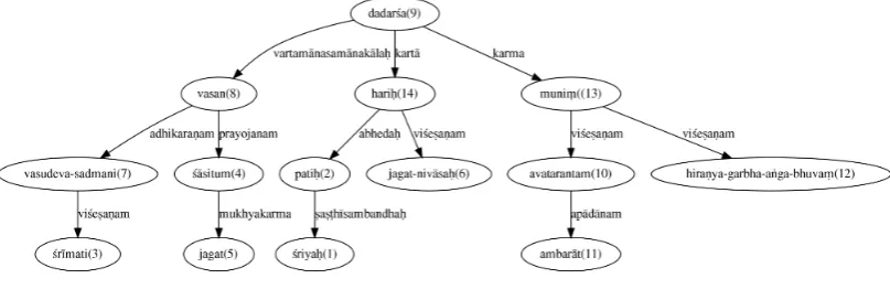
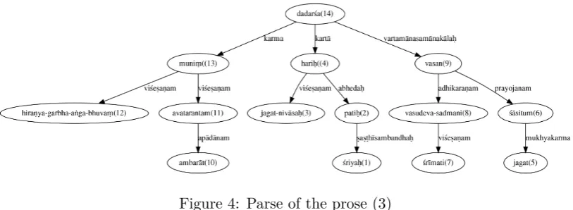
Figure 3 shows the parse of the first śloka from Śiśupālavadham by the poet Māgha, which occupies a prominent place among the Mahākāvyas. It has the three virtues of the best Kāvya, viz. upamā of Kālidāsa, arthagauravam of Bhāravi and padalālityam of Daṇḍi. We also tried to parse the daṇḍa-anvaya of the same śloka, and Figure 4 shows the parse of the anvaya. The śloka and its prose form are given below.

Śloka: śriyaḥ patiḥ śrīmati śāsituṁ jagat jagat-nivāsaḥ vasudeva-sadmani |

vasan dadarśa avatarantaṁ ambarāt hiraṇya-garbha-aṅga-bhuvaṁ muniṁ hariḥ || (2)

Daṇḍa-anvaya: śriyaḥ patiḥ jagat-nivāsaḥ hariḥ jagat śāsituṁ śrīmati vasudeva-sadmani vasan ambarāt avatarantaṁ hiraṇya-garbha-aṅga-bhuvaṁ muniṁ dadarśa | (3)

Eng: Lakṣmi’s consort,Viṣṇu, who is the source of the world, who was residing in the house of Vasudeva to control the world, saw Brahma’s son Nārada, descending from the sky.

Figure 4: Parse of the prose (3)

As stated earlier, our parser produces all possible parses, and since the constraint of mutual compatibility (yogyatā) is not yet implemented fully,6 _{the number of parses is on higher side.} The total number of parses produced by the machine, in the case of śloka and prose are 98,658 and 10,804 respectively. And the correct parse was found at 47,848th and 1,256th position respectively. The explanation for almost 10 fold increase in the number of parses in the case of śloka is as follows: In the case of prose, it is assumed that the head is to the right. So all the adjectives, and also the arguments of the predicate occur to the left of the head. But in the case of a śloka this condition does not hold. The adjectives as well as the arguments of the predicates can occur on either side of the head. Further, the adjectives and the modifiers with genitive case have more flexibility over the predicate-argument relations. Since they can cross the clausal boundaries, and that we have not yet implemented the meaning compatibility check on these relations, the possible number of solutions grows rapidly. Thus we notice that this parser can be still improved at two levels: a) To reduce the number of solutions. Study of mutual congruity among the meanings would help pruning out non-solutions. However, the representation of meaning congruity useful from computational point of view is challenging. b) The number of parses grow exponentially with the śloka order, and this is essentially because of the dislocation of adjectives and the genitives. More research is needed in order to understand the nature of dislocations and also syntactic constraints on such dislocations.

4 Understanding Texts: Commentary Tradition

In this section, we explain how the parsed structure can help us in understanding the original text in the same way as does the commentary tradition. Free word order in Sanskrit had a key role in the emergence of the poetic style, rather than prose, as a natural style for Sanskrit compositions. Authors who have written Sanskrit prose also have taken advantage of the free word order to present texts that are consistent with the intended meter or are interesting from the aesthetics point of view. But it is also true that it is difficult to understand poetry compared to prose. This is evident from the fact, we notice, that the commentators, especially commenting on the kāvya (poetic) literature, first rewrite the verse in prose in some default word order, and then comment on it. This deviation from the normal word order adds an extra load on the part of the readers in understanding the poetry. In order to understand such texts, one needs special training for interpreting these texts. We come across commentaries on several of such Sanskrit poetic texts, which make their understanding easier.

In the Indian tradition, we see two methods followed by commentators while dealing with sentence level analysis of ślokas (Tubb and Boose, 2007). In both these approaches, the aim of the commentator is to unfold the encoded meaning. While doing so, the commentator takes clues from the theories of śābdabodha. The two approaches are described below.

• The first approach is known as Khaṇḍa-anvaya (also known as katham-bhūtinī), where the commentator starts with the verb, and the expectancies associated with the verb, and goes

on filling these slots with the nominal forms in the śloka. Once the basic skeleton with all the expectancies is ready, then the commentator connects the viśeṣaṇas (adjectives) to their viśeṣyas (headwords), providing flesh to the skeleton.

The parse produced by the machine provides us the khaṇḍānvaya. All the words that are directly related to the verb work as a backbone, or as a part of the sentence carrying core information. The adjectives attached to the nouns, the arguments of non-finite verbs, etc. typically occupy the second or higher level in the tree structure, and add the flesh to the structure.

• The second approach is the Daṇḍa-anvaya (also known as anvaya-mukhī). In this method, first the commentator arranges the words in the śloka in a prose form, following a default word order typically encountered in prose.

In the next section, we present an algorithm that produces the Daṇḍa-anvaya for a śloka, from its parsed output.

5 Daṇḍa-anvaya-janaka

The dependency structure, produced by the parser described above, of the following śloka from Bhagavadgītā is shown in Figure 5.

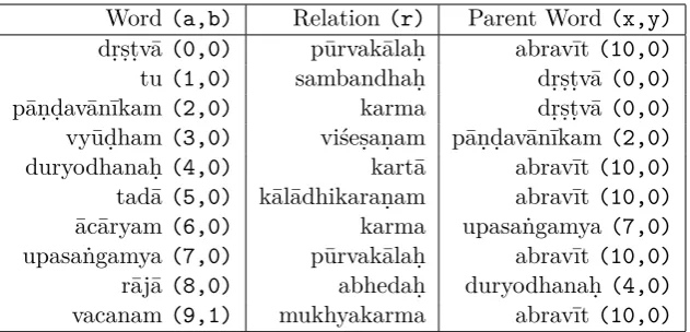
Dṛṣṭvā tu pāṇḍavānīkam Vyūḍham duryodhanaḥ tadā | Ācāryam upasaṅgamya Rājā vacanam abravīt || (BhG 1.2)

At that time, after seeing the army of the Pāṇḍavas arranged in military phalanx, Duryodhana approached (his) teacher and spoke (these) words.

Figure 5: Dependency graph of Bhagavadgita 1.2 śloka

The machine internal representation of this parsed output is in the form of a set of quintuplets containing the relations among words. Each quintuplet(a, b, r, x, y)consists of information about one dependency relation where,

a represents the word ID

b represents the morphological variant of the word

r represents the relation of the word with its parent word x represents the word ID of the parent word

Word (a,b) Relation (r) Parent Word (x,y)

dṛṣṭvā (0,0) pūrvakālaḥ abravīt(10,0)

tu (1,0) sambandhaḥ dṛṣṭvā (0,0)

pāṇḍavānīkam (2,0) karma dṛṣṭvā (0,0)

vyūḍham (3,0) viśeṣaṇam pāṇḍavānīkam (2,0)

duryodhanaḥ (4,0) kartā abravīt(10,0)

tadā(5,0) kālādhikaraṇam abravīt(10,0)

ācāryam (6,0) karma upasaṅgamya(7,0)

upasaṅgamya(7,0) pūrvakālaḥ abravīt(10,0)

rājā (8,0) abhedaḥ duryodhanaḥ (4,0)

vacanam (9,1) mukhyakarma abravīt(10,0)

Table 3: Output of Samsaadhanii parser

Table 3 shows the machine internal representation of the dependency graph shown in Figure 5. The shared roles are marked by dotted lines. For the purpose of re-ordering the words in Daṇḍa-anvaya order, these shared roles are not useful and hence ignored.

Initializing Reordering Task

Anvaya reordering tool is a simple script written in Python. It takes the set of quintuplets as input and creates a corresponding Python tree object. Since multiple morphological variants of a word cannot occur in a single set of dependency solution, variant information is not used presently but is preserved for proposed uses in the future.

Graphical representation of the tree object created with the parsed information of the Bha-gavadgītā verse is same as in Figure 5, without the dotted lines.

Deciding the Order

We found the clues for anvaya-order in the Samāsacakra. The two relevant kārikās go like this.

Ādau kartṛpadam vācyam dvitīyādipadam tataḥ Ktvātumunlyap ca madhye tu kuryād ante kriyāpadam (Samāsacakram kārikā 4, (Bhagirath, 1901, p. 12))

Starting with kartṛ, followed by other words, placing the non-finite verbal forms such as ktvā, tumun,lyapin between, place the main verb at the end.

Viśeṣaṇam puraskṛtya viśeṣyam tadanantaram Kartṛ-karma-kriyā-yuktam etad anvaya-lakṣaṇam (Samāsacakram kārikā 10, (Bhagirath, 1901, p. 13))

Starting with adjectives, targeting the headword, in the order of kartṛ-karma-kriyā (subject-object-verb), gives an anvaya (the natural order of words in a sentence).

In recent studies, Aralikatti (1991) has shown that the unmarked word order in Sanskrit is SOV. That is, all the arguments of a verb are placed to the left of the verb starting with the kartṛ, then karman followed by other arguments, the attributive adjectives are placed to the left of the noun they qualify, and the predicate is at the end of the sentence. The sub-ordinate clauses, if any, are before the predicate.

Taking clue from these resources, we define a sentence to be in canonical word orderif it satisfies the following criteria:

All the modifiers are placed to the left of the word they modify.

This is equivalent to the following.

1. The adjectives are to the left of the substantives they qualify.

3. All the non-finite forms that modify the finite verb form are to its left.

This implies that the main verb7 is always the last word of a sentence. This canonical word order provides us the Daṇḍa-anvaya for ślokas. We assigned the priorities to the dependency relation labels following these clues. These priorities were further fine-tuned by studying the commentaries and prose orders of around 400 ślokas from literature including Bhagavadgītā, Nītiśataka, various subhāṣitas and about 50 poetic prose sentences from Kādambarī.

Adjusted by various measures, currently, the relative positions of various arguments are fixed following the rules given below.

1. Sambodhya (vocative) comes at the initial position in the canonical order. 2. Kartṛ comes after vocative.

3. Kāraka relations follow in reverse order i.e. adhikaraṇa, apādāna, sampradāna, karaṇa and karman.

4. Viśeṣanas, modifiers with genitive case markers, etc. are placed before their viśeṣya. 5. Kriyāviśeṣana, pratiṣedha etc. are placed immediately before their corresponding verb. 6. Mukhyakriyā is positioned at the end of the sentence.

7. Avyaya particles such astu and api are placed immediately after their parent word. 8. The non-finite verbal forms are placed before the karman. All the arguments of non-finite

verb appear to their left.

9. The kartṛ-samānādhikaraṇa and karma-samānādhikaraṇa are placed after the katṛ and karman respectively.

Sorting the Tree

The reordering tool traverses through the tree object using level-order-iteration and sort re-cursively at each node. Primary sorting is carried out based on the relation priorities. The indeclinables such as emphatic particles, and conjuncts are left out as their positions are fixed with respect to their parent node. If there are relations with equal priorities at any level, secondary sorting is done based on the word order (ID) in the original sentence.

The reordered dependency tree of the example śloka is represented in Figure 6.

Figure 6: Dependency tree object with sorted relations

Linearizing the Tree

The sorted dependency tree is linearized to get the anvaya order. The tree is traversed using post-order-iteration and each node is added to the linear order pattern.

7_{The main verb can be either in finite form, or in a participial form with either of the suffixes: kta,ktavatu}

The tree mentioned in Figure 6 is linearized in the order: Rājā Duryodhanaḥ vyūḍham pāṇḍavānīkam dṛṣṭvā tu ācāryam upasaṅgamya tadā8 vacanam abravīt.

5.1 Performance

This parser was tested on 195 instances and their canonical prose versions. The sample was taken from the corpus available at Heritage Platform9_{, which essentially corresponds to the citations} in the dictionary entry and thus is a random selection from Sanskrit texts belonging to different branches of knowledge and different time period. We provided manually their canonical form. And both the canonical form as well as verse form was run through the parser. Out of 195, the parser could not parse 45 instances both in prose as well as in verse form. One major reason for the failure is out of vocabulary words. The average number of parses for verse order text and prose order text were 151 and 60 respectively. There were around 10 instances, where the number of parses was greater than 1000. This was mainly due to over-analysis with the genitive case markers, in the absence of proper handling of mutual congruity. The median for number of parses is 4, for both verse as well as prose.

Some of the limitations of the current parser are—

1. The parser is based on the Vaiyākaraṇa’s theory of śābdabodha. As such, it expects a verb in a sentence. Sanskrit has a tendency of eliding stative verbs meaning ‘to be’ like asti, bhavati etc. Parser shows poor performance dealing with such sentences.

2. The relation of kartṛsamānādhikaraṇa is established with a noun, only if it agrees with kartṛ in gender, number, person and case suffix. There are exceptions in literature where samānādhikaraṇas have semantic compatibility though they don’t agree in gender, number etc. For example,

• Chandaḥ pādau tu vedasya (chandaḥand pādau do not agree in number).

• Māyā idam sarvam (Gender ofmāyā does not agree with that ofidam and sarvam). Parser fails to establish relations among such words.

3. Parser performs poorly on some domain specific sentences. Here is an example from math-ematical domain: caturādhikam śatamaṣṭaguṇam dvāṣaṣṭistathā sahasrāṇām ayutadvaya-viṣkambhasyāsannaḥ vṛttapariṇāhaḥ.

6 Conclusion

The main purpose behind the development of an indegenous parser was to evaluate the usefulness of the theories of śābdabodha for the mechanical parsing of Sanskrit sentences. The theories of śābdabodha discuss in minute detail the flow of information, various means of encoding the information, the amount of information encoded, and so on. These theories were further supported by providing various conditions such as ákāṅkṣā, yogyatā and sannidhi, that help in the process of verbal cognition. So we decided to model these conditions computationally.

In this paper we have presented an edge-centric algorithm that handles both prose as well as poetry. In this algorithm, the incompatibility between the edges is noticed at an early stage. And hence the non-solutions are thrown out at an early stage. The user interface allows the user to select the best suited segmentation and provide the canonical word order of such segmented text.

We noticed that the performance of the algorithm when the input is in prose form is better than when it is in verse form. The relations contributing to the over-generation are the relation due to genitive case suffix and the adjectival relation. More research towards the nature of dislocation and syntactic constraints on dislocation, and also the semantic compatibility of the words related thus would help in rejecting the non-solutions mechanically.

8_{Here tadā, though a kālādhikaraṇam, acts as a connector between the previous and the current sentence,}

and thus should be at the beginning of a sentence. However, since the current implementation does not handle inter-sentential relations, the word ‘tadā’ is not placed at the beginning.

References

[Aralikatti1991] R. N. Aralikatti. 1991. A note on word order in modern spoken Sanskrit and some positive constraints. In Hans Henrich Hock, editor, Studies in Sanskrit Syntax, pages 13–18. Motilal Banarsidass Publishers.

[Attardi2006] Giuseppe Attardi. 2006. Experiments with a multilanguage non-projective dependency parser. In Proceedings of CoNLL, pages 166–170.

[Bhagirath1901] Hariprassad Bhagirath. 1901. Samāsacakra. Jagadishwar Press, Mumbai.

[Delmonte2018] Rodolfo Delmonte. 2018. Syntax and semantics of italian poetry in the first half of the 20th century. arXiv:1802.03712v2 [cs.CL].

[Gillon1993] Brendan S. Gillon. 1993. Bhartṛhari’s solution to the problem of asamartha compounds. Études Asiatiques/Asiatiche Studien, 47(1):117–133.

[Gillon1996] Brendan S. Gillon. 1996. Word order in Classical Sanskrit. Indian Linguistics, 57(1):1–35.

[Joshi1968] S. D. Joshi. 1968. Patañjali’s Vyākaraṇa-mahābhāṣya. Samarthāhnika. Edited with translation and explanatory Notes. Center of Advanced Study in Sanskrit. Class C, No. 3. University of Poona, Poona.

[Krishna et al.2019] Amrith Krishna, Vishnu Sharma, Bishal Santra, Aishik Chakraborty, Pavankumar Satuluri, and Pawan Goyal. 2019. Poetry to prose conversion in sanskrit as a linearisation task: A case for low-resource languages. forthcoming.

[Kulkarni et al.2010] Amba Kulkarni, Sheetal Pokar, and Devanand Shukl. 2010. Designing a constraint based parser for Sanskrit. In G. N. Jha, editor, Proceedings of the Fourth International Sanskrit Computational Linguistics Symposium, pages 70–90. Springer-Verlag LNAI 6465.

[Kulkarni et al.2015] Amba Kulkarni, Preeti Shukla, Pavankumar Satuluri, and Devanand Shukl. 2015. How free is the ‘free’ word order in Sanskrit. In Peter Scharf, editor, Sanskrit Syntax, pages 269–304. Sanskrit Library.

[Kulkarni2013] Amba Kulkarni. 2013. A deterministic dependency parser with dynamic programming for Sanskrit. InProceedings of the Second International Conference on Dependency Linguistics (DepLing 2013), pages 157–166, Prague, Czech Republic, August. Charles University in Prague Matfyzpress.

[Kulkarni2019] Amba Kulkarni. 2019. Sanskrit Parsing based on the theories of śābdabodha. D. K. Printworld and Indian Institute of Advanced Studies, Delhi.

[Lee and Kong2012] John Lee and Yin Hei Kong. 2012. A dependency treebank of classical Chinese poems. In Conference on North American Chapter of the Association of Computational Linguistics: Human Language Technologies, pages 191–199.

[Lin1998] Dekang Lin. 1998. Dependency-based evaluation of minipar. InWorkshop on the Evaluation of Parsing Systems, Granada, Spain.

[Mcdonald and Nivre2007] Ryan Mcdonald and Joakim Nivre. 2007. Characterizating the errors of data-driven dependency parsing models. In Proceedings of EMNLP-CoNLL, pages 122–131.

[McDonald et al.2005] Ryan McDonald, Fernando Pereira, Kiril Ribarov, and Jan Hajiç. 2005. Non-projective dependency parsing using spanning tree algorithms. InProceedings of HLT/EMNLP, pages 523–530.

[Nakagawa2007] Tetsuji Nakagawa. 2007. Multilingual dependency parsing using global features. In Proceedings of the Joint Conference on EMNLP-CoNLL.

[Nivre and Scholz2004] J. Nivre and M. Scholz. 2004. Deterministic dependency parsing of english text. InProceedings of COLING 2004, pages 64–70, Geneva, Switzerland.

[Panchal and KulkarniJuly 2018] Sanjeev Panchal and Amba Kulkarni. July 2018. Yogyataa as an ab-sence of non-congruity. In Gérard Huet and Amba Kulkarni, editors, Computational Sanskrit and Digital Humanities, selected papers presented at the 17th world Sanskrit Conference, Vancouver. D. K. Publishers and Distributors Pvt. Ltd.

[Scharf et al.2015] Peter Scharf, Anuja Ajotikar, Sampada Savardekar, and Pawan Goyal. 2015. Dis-tinctive features of poetic syntax preliminary results. In Sanskrit Syntax, pages 305––324. Sanskrit Library, USA.

[Sleator and Temperley1993] Daniel D. Sleator and Davy Temperley. 1993. Parsing english with a link grammar. InThird International Workshop on Parsing Technologies.

[Speijer1886 Reprint 2009] J. S. Speijer. 1886; Reprint 2009. Sanskrit Syntax. Motilal Banarsidass, New Delhi.

[Tubb and Boose2007] Gary A. Tubb and Emery R. Boose. 2007. Scholastic Sanskrit: A Handbook for students. The American Institute of Buddhist Studies at Columbia University in the City of New York, New York.