Human Language Technologies: The 2009 Annual Conference of the North American Chapter of the ACL, pages 530–538,
Semantic-based Estimation of Term Informativeness
Kirill Kireyev
University of Colorado – Boulder
[email protected]
Abstract
The idea that some words carry more semantic content than others, has led to the notion of term specificity, or informativeness. Computa-tional estimation of this quantity is important for various applications such as information re-trieval. We propose a new method of comput-ing term specificity, based on modelcomput-ing the rate of learning of word meaning in Latent Semantic Analysis (LSA). We analyze the performance of this method both qualitatively and quantitat-ively and demonstrate that it shows excellent performance compared to existing methods on a broad range of tests. We also demonstrate how it can be used to improve existing applica-tions in information retrieval and summariza-tion.
1
Introduction
The idea that some words carry more semantic content than others has been occurring in various literature in linguistics, psychology and computer science for some time. The intuitive notion of
spe-cificity has long existed before it was formalized;
consider, for example, the distinction between the more general word “beverage” and more specific terms “tea”, “coffee” and “cocoa” made by Spär-ck-Jones (1973). Another informal mention of spe-cificity is mentioned by Gorman (1961):
A word may be “abstract” and either general or specific, or “concrete” and either general or specific.
where it is contrasted with another psycholinguistic property of concreteness, which is generally defined as “the extent to which the word's referent can be touched or felt” (Reilly et al., 2007).
The field of information retrieval has attracted greater attention to the computational estimation and applications of term specificity. It has been noted that words with higher specificity, or
inform-ation content, deserve to be weighted more heavily
when matching documents with queries, since
these words play a greater importance in character-izing what a query or a document is about. By con-trast, stopwords, words that contribute the least amount of semantic content, are often down-weighted or removed altogether (see (Lo et al., 2005), for example).
In addition to IR, term specificity, or informat-iveness, has been shown useful in other applica-tions, such as Named Entity Tagging (Rennie et al., 2005), creating back-of-the-book glossaries (Csomai et al., 2007), and extractive summariza-tion (Kireyev, 2008).
A related notion of communication density has been introduced by Gorman et al. (2003) in team communication analysis, to measure the extent to which a team conveys information in a concise manner, or, in other words, the rate of meaningful discourse, defined by the ratio of meaningfulness
to number of words spoken. The meaningfulness
described here should not be confused with psy-cholinguistic quality of meaningfulness as de-scribed by Toglia and Battig (1978), which is the degree to which a word is associated with other words.
In this paper we consider the terms specificity,
informativeness and information content of words
to mean the same thing. A precise formulation or analysis of important qualitative characteristics of these concepts has not been performed in previous literature; we hope to make some progress in that direction in this paper.
Our main goal is to introduce a new method of computing word specificity based on the rate and strength of semantic associations between words, as modeled by Latent Semantic Analysis (LSA).
2
Previous Approaches
To date, most of the known approaches to estim-ating term informativeness have relied on fre-quency-based methods.
A very basic, yet surprisingly effective approach to measuring term informativeness is its frequency of occurrence in a large representative corpus of language. Spärck Jones (1973) defines IDF or
in-verse document frequency, which is determined by
the probability of occurrence of documents con-taining a particular word:
IDFw=−log2dfw/D
where D is the total number of documents in the corpus. The assumption behind it is that low fre-quency words tend to be rich in content, and vice versa.
Church and Gale (1995) correctly note that this measure is fundamentally different from collection
frequency fw, (the total number of times the word
type occurs in the corpus) or its transformations, despite the fact that the two measures appear highly correlated. In fact, what is particularly of in-terest are the words for which these two quantities deviate the most. This happens most dramatically for most informative, or content words, such as “boycott” (Church, 1995a).These words happen to exhibit “bursty” behavior, where they tend to ap-pear multiple times but in fewer documents, thus having fw > dfw. In contrast, less content-loaded words like “somewhat” tend to occur on average once in documents, and thus have similar values for collection and document frequencies ( fw ≈ dfw ). As a result, more informative words can be less ac-curately estimated by the Poisson distribution, which is based on the simplistic assumption that the expected number of occurrences of word in a document can be estimated by its total number of occurrences in the corpus.
Most prominent statistical measures of term in-formativeness rely on quantifying this notion of deviation from the Poisson distribution. If the mean expected word rate is:
t
w=
f
wD
then the variance metric can be defined as:
variance
w
=
1
D
−
1
∑
d=1D
t
dw−
t
w
2where tdw is the actual number of occurrences of term w in document d. The idea is that a higher variance would indicate greater deviation from
ex-pected frequency of occurrence in a document, which is assumed to be higher for informative words.
Another measure, suggested by Church and Gale (1995a) is burstiness which attempts to com-pare collection frequency and document frequency directly:
burstiness
w
=
t
wdf
w/
D
=
f
wdf
wChurch and Gale also noted that nearly all words have IDF scores that are larger than what one would expect according to an independence-based model such as the Poisson. They note that interest-ing or informative words tend to have the largest deviations from what would be expected. They thus introduce the notion of residual IDF which measures exactly this deviation:
residualIDF
w
=
IDF
w
log
2
1
−
e
−t
Papineni (2001) introduces the notion of gain:
gain
w
=
df
wD
df
wD
−
1
−
log
df
wD
This measure tends to give low weights to very high- and very low- frequency words.
Most closely related to our work is the notion of
meaningfulness in (Gorman et al 2003), computed
as the LSA vector length. We will discuss it further in the subsequent sections, and show that a small but crucial modification to this quantity gives the best results.
3
Using Latent Semantic Analysis for
Ap-proximating Term Informativeness
3.1 Latent Semantic Analysis
all of the words can be represented as vectors. The number of dimensions is then artificially reduced to a smaller number (typically around 300) of most important dimensions, which has the effect of smoothing out incidental relationships and pre-serving significant ones between words.
The resulting geometric space allows for straightforward representation of meaning of words and/or documents; the latter are simply a weighted geometric composition of constituent word vectors. Similarity in meaning between a pair of words or documents can be obtained by comput-ing the cosine between their correspondcomput-ing vectors. For details of LSA, please see (Landauer et al., 2007), and others
3.2 LSA Term Vector Length
Most of the LSA applications focus on compar-ing semantic similarity between words and/or text, using the cosine measure of the angle between the corresponding vectors. There is, however, another significant characteristic of LSA word vectors be-sides their direction in space; it is their vector length. The vector length for words differs signi-ficantly, as is shown in Table 1.
Word dfw Vector Length
dog 1365 1.3144
green 2067 0.7125
run 2721 0.4788
puppy 127 0.2648
electron 264 0.9009
[image:3.612.323.513.505.608.2]the 44474 0.0098
Table 1: LSA vector length for some of the words in TASA corpus.
The vector length plays a very important role in many LSA calculations, in particular – in giving relative weights to the word vectors that constitute a particular text passage.
What causes differences in vector lengths? They are based roughly on how much information LSA learns about a word based on its patterns of occur-rence in the corpus. Kintsch (2001) writes:
Intuitively, the vector length tells us how much in-formation LSA has about this vector. [...] Words that LSA knows a lot about (because they appear fre-quently in the training corpus[...]) have greater vector lengths than words LSA does not know well. Func-tion words that are used frequently in many different contexts have low vector lengths -- LSA knows
noth-ing about them and cannot tell them apart since they appear in all contexts.
Essentially, there are two factors that affect vec-tor length: (1) number of occurrences and (2) the consistency of contexts in which the word occurs.
3.3 Deriving Specificity from Vector Length Based on the observations above we propose a new metric of term informativeness, or specificity, which we call LSAspec, which is simply the ratio of LSA vector length to the number of documents in the LSA training corpus that contain a particular word:
LSAspec
w
=∥
w
∥/
df
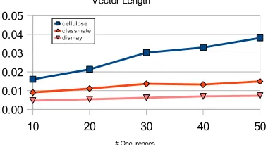
wThe value can be interpreted as the rate of vector length growth. We argue that more specific, or in-formative, words have the greatest rate of vector length growth; LSA learns about their meaning faster, with relatively fewer exposures. To illus-trate this concept, let's look at a few examples, that were obtained by controlling the number of occur-rences of a particular word in the LSA training cor-pus. The base corpus was obtained using the 44000-passage TASA corpus with all passages containing the three words below initially re-moved. Each data point on the graph reflects the vector length of a particular word, after training LSA on the base corpus plus the specified number of passages containing a particular word added back. Highly specific words like “cellulose” gain vector length quite quickly compared to a low-spe-cificity word like “dismay”.
4
Comparison of Specificity Metrics
Past attempts to examine the merits of various existing term informativeness estimation methods in the literature thus far has largely involved
em-Illustration 1: Vector lengths for some words vs the number of documents containing those words.
10 20 30 40 50
0.00 0.01 0.02 0.03 0.04 0.05
Vector Length
cellulose classmate dismay
pirical summative evaluations as part of informa-tion retrieval or named entity tagging systems (Rennie et al., 2005). Here, we provide some measures which hopefully provide more illuminat-ing insights into the various methods.
In all of the tests below we derived the metrics (including the LSA space for LSAspec) from the same corpus – MetaMetrics 2002 corpus, com-posed of ~188k passages mostly used in education-al texts. No stemming or stopword removeducation-al of any kind was performed. All word types were conver-ted to lowercase. We compuconver-ted the specificity score for each of the 174,374 most frequent words in the corpus using each of the metrics described above: LSAspec, IDF, residualIDF, burstiness, gain and variance.
4.1 Correlation with Number of Senses
Intuitively, one would expect more specific words to have more precise meaning, and there-fore, generally fewer senses. For example, “elec-tron” is a specific physics term that has only one sense, whereas “run” has a very general meaning, and thus has over 50 senses in the WordNet data-base (Miller et al., 1990). There are many excep-tions to this, of course, but overall, one would ex-pect a negative correlation between specificity and number of senses.
In this test, we measure the correlation between the specificity score of a word by various methods and its number of senses in WordNet version 3.0. A total of 75,978 words were considered. We use Spearman correlation coefficient, since the rela-tionships are likely to be non-linear.
Metric Corr Metric Corr
LSAspec -0.46 burstiness -0.02
IDF -0.44 variance 0.40
residualIDF -0.03 gain 0.44
Table 2: Correlation of specificity metrics with number of senses in WordNet
LSAspec gives the highest negative correlation
with number of WordNet senses.
4.2 Correlation with Hypernymy
WordNet organizes concepts into a hypernymy tree, where each parent node is a hypernym of the child node below it. For example:
substance
element
metal
nickel copper
In general one would expect that for each pair of child-parent pairs in the hypernym tree, the child will have greater specificity than the parent1. We
examined of a total of 14451 of such hypernym word pairs and computed how often the child's in-formativeness score, according to each of the measures, is greater than its parent's (its hyper-nym's) score.
Metric Percent Metric Percent
IDF 88.8% burstiness 47.2%
LSAspec 87.7% variance 13.4%
residualIDF 48.8% gain 11.1%
Table 3: Percentage of the time specificity of child ex-ceeds that of its hypernym in WordNet
4.3 Writing Styles and Levels
One may expect that the specificity of words on average would change with texts that are known to be of different writing styles and difficulty level. To test this hypotheses we extracted texts from the TASA collection of educational materials. The texts are annotated with genre (“Science”, “Social Studies” or “Language Arts”), and difficulty level on the DRP readability scale (Koslin et al., 1987). Intuitively, one would expect to see two patterns among these texts:
(1) The specificity of words would generally in-crease with increasing level of difficulty of texts.
(2) Informative (Science) texts should have more specific terms than narrative (Language Arts) texts; with Social Studies somewhere in between (McCarthy et al., 2006).
We extracted 100 text passages for each com-bination of style (“Science”, “Social Studies”, “Language Arts”) and DRP difficulty level (50, 55, 60, 65, 70)2, thus resulting in 15 batches of 100
passages. For each passage we computed the medi-an specificity measure of each unique word type in
1 In practice this is more difficult to determine, since some
Word-Net entries are actually phrases, rather than words (e.g. “tulip” ← “liliaceous plant” ← ... ← “plant”). In such cases we search up the tree until we stumble upon a node where the entry (or one of the entries) is a single word.
2 DRP level of 50 roughly corresponds to the beginning of 6th grade
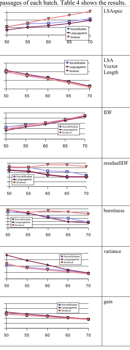
the passage, and averaged these values over 100 passages of each batch. Table 4 shows the results.
LSAspec
LSA Vector Length
IDF
residualIDF
burstiness
variance
[image:5.612.72.297.80.683.2]gain
Table 4: Average median specificity scores for texts of different genres and DRP levels.
Note that the absolute values for a particular batch of texts are not important in this case; it's the relative differences between batches of different styles and difficulty levels that are of interest. Of all the measures, only LSAspec appears to exhibit the two characteristics described above (increasing with text difficulty, and separating the three genres in the expected way). The metrics residualIDF and
burstiness also appear to separate the genres as
ex-pected, but they do not increase with text diffi-culty.
It is also evident that LSA Vector Length alone does not serve as a good measure of informative-ness, contrary to its use as such in (Gorman et al., 2003). In fact, it shows the most dramatic and reli-able inverse relationship with text difficulty. This is likely due to the fact that texts of lower diffi-culty use common (easier) words more often; these words tend to have longer LSA vector lengths.
4.4 Back-of-the-Book Glossary
Educational textbooks typically have a glossary (index) at the end which lists important terms or concepts mentioned in the book. One would expect these terms to have greater informativeness com-pared to other words in the textbook. This was a crucial assumption used by Csomai and Mihalcea (2007), who used informativeness (as measured by
IDF and other metrics) as one of the main features used to automatically generate glossaries from textbooks.
We can use existing textbooks and their glossar-ies to validate this assumptions, by observing the extent to which the words in the glossary are ranked higher by different specificity metrics com-pared to other words. Note that the goal here is not to actually achieve optimal performance in auto-matically finding glossary words; for this reason we do not use recall/precision- based evaluation or rely on additional features such as term frequency (or the popular tfw∙idfw measure). Rather the goal is to simply see how much the glossary words exhibit the property (informativeness) that we are trying to compute with various methods.
We obtained a collection of textbook chapters (middle-school level material from Prentice Hall Publishing) and their corresponding glossaries, in two different genres: 8 on World Studies (e.g. “Africa”, “Medieval Times”) and 13 on Science (e.g. “Structure of Animals”, “Electricity”). Each 50 55 60 65 70
SocialStudies LanguageArts Science
50 55 60 65 70
SocialStudies LanguageArts Science
50 55 60 65 70
SocialStudies LanguageArts Science
50 55 60 65 70
SocialStudies LanguageArts Science
50 55 60 65 70
SocialStudies LanguageArts Science
50 55 60 65 70
SocialStudies LanguageArts Science
50 55 60 65 70
chapter was converted into text and a list of unique words was extracted.
For each of the specificity metrics, we compute how well it predicts glossary words:
1. Compute the specificity of each word in a chapter, according to the metric.
2. Order all the words in decreasing order of specificity.
3. Compute the median percentile rank (posi-tion) in the list above of all single-word entries in the glossary (top word has the rank of 0; bottom has a rank of 100). If a specificity metric predicts the glossary words well, we would expect the average rank to be low; i.e. glossary words would be near the top of the specificity-ordered list.
Metric Word Studies
(~9000 total wds / ch ~260 gloss wds / ch)
Science
(~1000 total wds / ch ~20 gloss wds / ch)
LSAspec 0.21 0.10
residualIDF 0.21 0.11
burstiness 0.21 0.12
IDF 0.29 0.16
variance 0.49 0.64
[image:6.612.319.537.438.572.2]gain 0.51 0.68
Table 5: Average median rank of glossary words among all other words in textbook by specificity.
LSAspec shows the lowest median percentile for
both genres of books.
4.5 Qualitative Analysis
It is useful to inspect the significant differences between the word rankings by different methods, to see if some notable patterns emerge. We can find words on which the methods disagree most dramatically by observing which of them have the most significant differences of position (0-100) in the word lists ranked by different specificity met-rics. To avoid dealing with overly-rare words, we restrict our attention to the 23,000 most frequent words in the corpus.
Let's first compare LSAspec and residualIDF. From the list of 100 words with the most extreme disagreements, we select some examples that have high rank for LSAspec (and low for residuaIDF)
and vice-versa. From Table 6 we can see that
re-sidualIDF misses some term words (such as
“chro-matin”) which LSAspec correctly rates as highly-specific words. Conversely, residualIDF,
incor-rectly ranks common words like “her” and “water” as highly-specific. The reason for this behavior is that words like “chromatin” happen to occur only once per document in the texts they are mentioned (e.g. dfcromatin = tfchromatin = 7), whereas “her” and “school” tend to occur frequently per document. In real applications “her” will probably be discarded using stopword lists, but “school” will probably not.
Word LSAspec residualIDF
oviducts 0.5 98.8
cuspids 0.6 98.8
chromatin 0.7 98.7
disassembly 0.7 98.7
her 99.9 1.5
my 99.9 3.5
water 97.5 5.1
school 97.8 10.3
Table 6: Words ranked most differently by LSAspec and residualIDF
Comparing LSAspec and burstiness we see al-most the same pattern, which is not surprising, since burstiness and residualIDF work from the same assumptions that content words tend to occur multiple times but in fewer documents.
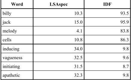
The table below lists examples of most notable differences between LSAspec and IDF.
Word LSAspec IDF
billy 10.3 93.5
jack 15.0 95.9
melody 4.1 83.8
cells 10.8 86.3
inducing 34.0 9.8
vagueness 32.5 9.6
initiating 31.5 8.7
apathetic 32.3 9.8
Table 7: Words ranked most differently by LSAspec and IDF and their percentiles
contrast, rare but vague words like “inducing” or “vagueness” are improperly given a high spe-cificity ranking.
5
Applications in LSA
Having demonstrated that our word specificity metric performs well with regards to some natural linguistic phenomena, we can now show that it can be used successfully as part of existing NLP tech-nologies. Here we will focus particularly on ap-plications within Latent Semantic Analysis (LSA), although it is highly likely that this specificity met-ric can be used successfully in other places as well. We will demonstrate that LSAspec shows better results that the conventional term weighting scheme in LSA. It is also important to note that al-though LSAspec is derived using LSA, it is in fact logically independent from the term weighting mechanism used by LSA; other metrics (such as the ones described above) could also be potentially used for LSA term weighting.
In order to represent the meaning of text in LSA, one typically computes the document vector of the text by geometric addition of word vectors for each of the constituent words:
V
d=
∑
w∈d
a
w∗
log
1
t
dw∗
v
wwhere aw is the log-entropy weight of the word
w, typically set to tfw∙idfw (or some variation there-of) , tdw is the number of occurrences of the word w
in the document, and vw is the vector of the word. Implicit in vw is its geometric length, which tends to be much greater for frequently-used words (un-less they are extremely vague). It is tempered somewhat by aw which is higher for content words, but perhaps not effectively enough, as the sub-sequent tests will show. McNamara et al. (2007) experimented with changing the weighting scheme, mainly focusing on prioritizing rare vs. frequent words, and has shown significant differ-ences in short-sentence comparison results.
In the sections below we compare the original LSA weighting scheme with our new scheme based on LSAspec:
V
d=
∑
w∈d
LSAspec
w
∗
log
1
t
dw∗
v
w∥
v
w∥
In other words, we replace the weight parameter aw and the implicit weight contained in the length of
each word vector (by normalizing it) with the spe-cificity value of LSAspec.
We show that the resulting term weighting scheme improves performance in three important applications: information retrieval, gisting and short-sentence comparison.
5.1 Information Retrieval
LSA was first introduced as Latent Semantic In-dexing (Deerwester et al, 1990), designed for the goal of more effective information retrieval by rep-resenting both documents and queries as vectors in a common latent semantic space.
In this IR context, the type of term weighting used to compose document and query vectors plays an important role. We show that using our
LSAspec-based term weighting gives superior
per-formance to the traditional weighting scheme de-scribed in the previous section.
We used the SMART Time3 dataset, a collection
of 425 documents and 83 queries related to Time magazine news articles. For this task only, we used a LSA space that was built using the AQUAINT-2 corpus4, a large collection (~440,000) of news
art-icles from prominent newspapers such as the New York Times. The variable parameter in the LSA IR models was the cosine threshold between the document and the query, which was varied between 0 and 1
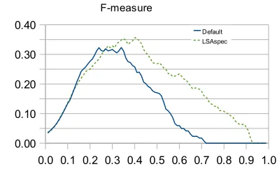
Figure 1 shows the performance of the original LSA and LSA with LSAspec5 term weighting method, in terms of the F-measure, which is the harmonic mean of precision and recall; a higher value means better performance. The abscissa in
3 ftp://ftp.cs.cornell.edu/pub/smart/time/
4 TREC conference: http://trec.nist.gov/
5 LSAspec measure was the same as before, derived from LSA built
[image:7.612.331.529.442.563.2]on MetaMetrics corpus.
Figure 2: The performance of default LSA and LSA+LSASpec on SMART IR dataset.
0.0 0.1 0.2 0.3 0.4 0.5 0.6 0.7 0.8 0.9 1.0 0.00
0.10 0.20 0.30 0.40
F-measure
the graph is the value of the threshold cosine para-meter. The LSAspec term weighting outperforms the original term weighting.
5.2 Sentence Similarity
Here we analyze performance of the two LSA term weighting methods on automated sentence similarity comparisons. Although LSA works best on units of text of paragraph-size or larger, it can work reasonably well on sentence-length units.
We use the dataset reported by McNamara (2007), where the authors collected a set of tence pairs from several books. A total of 96 sen-tence pairs was provided, consisting of a combina-tion of subsequent sentences in the book (16), non-adjacent sentences in the same book (16), tences from two different books (48), and sen-tences where one is a manually-created paraphrase of one another (16). The standard of reference for this task is human similarity ratings of these sen-tences within each pair, reported on a Likert scale between 6 (most similar) and 1 (completely dis-similar). Here we report correlations between hu-man rating and LSA similarity with the two term weighting metrics.
Original LSA: 0.66 LSA + LSAspec: 0.85
Using LSAspec term weighting gives better per-formance compared to the original LSA term weighting scheme.
5.3 Gisting (Very Short Summarization) The ability to represent documents and words in a common geometric space allows LSA to easily compute the gist of a document by finding the word (or sentence) whose vector is most similar by cosine metric to the document vector. This word can be interpreted as the most representative of the cumulative meaning of the document; it can also be thought as a one-word summary of the docu-ment. Gisting is discussed from a psychological perspective by Kintsch (2002).
Once again, the choice of term weighting mech-anism can make a significant difference in how the overall document vector is constructed. Here, we compare the original weighting scheme and
LSAspec in the performance on gisting. To perform
this evaluation, we selected 46 well-written Wiki-pedia6 articles in various categories: Sports,
Anim-als, Countries, Sciences, Religions, Diseases. The
6 http://en.wikipedia.org, circa May 2008.
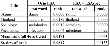
original single-word Wikipedia title of each of the articles can be thought as the optimal one-word gist of the article, thus serving as a reference an-swer in evaluation. A perfect gisting performance by the model would always select the original title as the closest word to the meaning of the docu-ment. We also measure the position of the original title in the list of all words in the article ranked by their similarity to the document vector, and ran-ging from 0 (original title picked as top word) and 1. Table 10 shows a few examples of both the top word and rank of the title, as well as the overall mean rank of all 46 articles.
Title Orig LSA LSA + LSAspec top word rank top word rank
Skiing skiing 0.0000 skiing 0.0000
Thailand buddhism 0.0189 thailand 0.0000
Sociology sociologists 0.0012 sociology 0.0000
Pneumonia infections 0.0064 infections 0.0092
[image:8.612.315.534.230.321.2]Mean rank (all 46 articles) 0.0191 0.0061 St. dev. of rank 0.0847 0.0133
Table 8: Examples of gisting (picking most representat-ive word for text) in with and without LSASpec in LSA
Using LSAspec noticeably improves gisting per-formance, compared to the original LSA term weighting method, as is evidenced by much lower mean rank of the original title.
6
Conclusion
We have introduced a new method of measuring word informativeness. The method gives good res-ults modeling some real linguistic phenomena, and improves LSA applications.
We attempted to look more deeply at the relev-ant characteristics of word specificity (such as cor-relation with number of senses). Our method seems to correspond with intuition on emulating a wide range of these characteristics. It also avoids a lot of pitfalls of existing methods that are based purely on frequency statistics, such as unduly pri-oritizing rare but vague words.
References
Kenneth W. Church and William A. Gale. 1995. Pois-son mixtures. Journal of Natural Language Engin-eering, 1995
Kenneth W. Church and William A. Gale. 1995a. In-verse document frequency (IDF): A measure of devi-ation from Poisson. In Proceedings of the Third Workshop on Very Large Corpora, pp 121–130, 1995.
András Csomai and Rada Mihalcea. 2007. Investiga-tions in Unsupervised Back-of-the-Book Indexing. In Proceedings of the Florida Artificial Intelligence Re-search Society, Key West.
Scott Deerwester, Susan T. Dumais, George W. Furnas and Thomas K. Landauer. 1990. Indexing by Latent Semantic Analysis. Journal of the American Society for Information Science, 41.
Aloysia M. Gorman. 1961. Recognition Memory for Nouns as a Function of Abstractness and Frequency. Journal of Experimental Psychology. Vol. 61, No. 1.
Jamie C. Gorman, Peter W. Foltz, Preston A. Kiekel and Melanie J. Martin. 2003. Evaluation of Latent Semantic Analysis-based Measures of Team Communication Content. Proceedings of the Human Factors and Ergonomics Society, 47th Annual Meet-ing, pp 424-428.
Walter Kintsch. 2002. On the notions of theme and top-ic in psychologtop-ical process models of text compre-hension. In M. Louwerse & W. van Peer (Eds.) Thematics : Interdisciplinary Studies, Amsterdam, Benjamins, pp 157-170.
Walter Kintsch. 2001. Predication. Journal of Cognitive Science, 25.
Kirill Kireyev. 2008. Using Latent Semantic Analysis for Extractive Summarization. Proceedings of Text Analysis Conference, 2008.
B. L. Koslin, S. Zeno, and S. Koslin. 1987. The DRP: An Effective Measure in Reading. New York College Entrance Examination Board.
Thomas K Landauer and Susan Dumais. 1997. A solu-tion to Plato's problem: The Latent Semantic nalysis theory of the acquisition, induction, and representa-tion of knowledge. Psychological Review, 104, pp 211-240.
Thomas K Landauer, Danielle S. McNamara, Simon Dennis, and Walter Kintsch. 2007. Handbook of Lat-ent Semantic Analysis Lawrence Erlbaum.
Rachel TszWai Lo, Ben He, and Iadh Ounis. 2005. Automatically Building a Stopword List for an formation Retrieval System. 5th Dutch-Belgium In-formation Retrieval Workshop (DIR). 2005.
Philip M. McCarthy, Arthur C. Graesser, Danielle S. McNamara. 2006. Distinguishing Genre Using Coh-Metrix Indices of Cohesion. 16th Annual Meeting of the Society for Text and Discourse, Minneapolis, MN, 2006.
Danielle S. McNamara, Zhiqiang Cai, and MaxM. Louwerse. 2007. Optimizing LSA Measures of Cohe-sion. Handbook of Latent Semantic Analysis . Mah-wah, NJ: Erlbaum. ch 19, pp 379-399.
George A. Miller, Richard Beckwith, Christiane Fell-baum, Derek Gross and Katherine Miller. 1990. WordNet: An on-line lexical database. International Journal of Lexicography, 3 (4), 1990.
Kishore Papineni. 2001. Why inverse document fre-quency. In Proceedings of the NAACL, 2001
Jamie Reilly and Jacob Kean. 2007. Formal Distinctive-ness Of High- and Low- Imageability Nouns: Ana-lyses and Theoretical Implications. Cognitive Sci-ence, 31.
Jason D. M. Rennie and Tommi Jaakkola. 2005. Using Term Informativeness for Named Entity Detection. Proceedings of ACM SIGIR 2005.
Karen Spärck-Jones. 1973. "A Statistical Interpretation of Term Specificity and its Application in Retrieval," Journal of Documentation, 28:1.