CLUZH at VarDial GDI 2017: Testing a Variety of Machine Learning Tools for the Classification of Swiss German Dialects

CLUZH at VarDial GDI 2017: Testing a Variety of Machine Learning

Tools for the Classification of Swiss German Dialects

Simon Clematide

Institute of Computational Linguistics University of Zurich

[email protected]

Peter Makarov

Institute of Computational Linguistics University of Zurich

[email protected]

Abstract

Our submissions for the GDI 2017 Shared Task are the results from three different types of classifiers: Na¨ıve Bayes, Condi-tional Random Fields (CRF), and Support Vector Machine (SVM). Our CRF-based run achieves a weighted F1 score of 65% (third rank) being beaten by the best sys-tem by 0.9%. Measured by classification accuracy, our ensemble run (Na¨ıve Bayes, CRF, SVM) reaches 67% (second rank) being 1% lower than the best system. We also describe our experiments with Recur-rent Neural Network (RNN) architectures. Since they performed worse than our non-neural approaches we did not include them in the submission.

1 Introduction

The goal of our participation in the newly intro-duced German Dialect Identification (GDI) Shared Task of the VarDial Workshop 2017 (Zampieri et al., 2017) was to quickly test how far we could get on this classification problem using standard machine learning techniques (as only closed runs were allowed for this task).

The task is to predict the correct Swiss Ger-man dialect for Ger-manually transcribed utterances (Samardzic et al., 2016).1 _{The Dieth}

transcrip-tion (Dieth, 1986)—developed in the 1930s in Switzerland—is not a scholarly phonetic tran-scription system. It is designed to be applicable by laymen to all Swiss German dialects and uses the Standard German alphabet and a few optional diacritics.

In this task, the number of possible Swiss Ger-man dialects is limited to four main varieties: the

1_{Since the text segments are transcribed speech, with a}

slight abuse of terminology, we shall refer to them as utter-ances.

dialects spoken in the cantons of Basel (BS), Bern (BE), Lucerne (LU), and Zurich (ZH).

The four approaches that we have worked on for this task are: i) a powerful baseline that uses an off-the-shelf Na¨ıve Bayes classifier trained on bags of character n-gram features; ii) an uncon-ventional yet effective application of a CRF clas-sifier to sequence classification—the system per-forming best on the official test set among all our runs; iii) a majority-vote ensemble of the Na¨ıve Bayes, CRF and SVM systems; and iv) an RNN character-sequence classifier trained on augmen-ted data, which however has not been included in our final submission.2

2 Related Work

Scherrer and Rambow (2010) describe dialect identification approaches to written Swiss Ger-man. To distinguish among six dialects, they ex-periment with a word n-gram model. Additionally, they attempt word-based identification by turning Standard German words into their dialectal forms according to hand-written transfer rules. They dis-cuss the linguistic aspects of the problem and dif-ficulties in predicting for the multitude and con-tinuum of Swiss German dialects.

Most of our final submission, except probably Run 2, is an application of well-established tech-niques for text classification (Sebastiani, 2002). We use regularized linear classifiers on a bag-of-character-n-grams representations of utterances. Despite its conceptual simplicity, this recipe pro-duces state-of-the-art results on language identi-fication tasks (Malmasi et al., 2016) and is par-ticularly easy to implement given the wide vari-ety of readily available tools for feature extraction and classification. Having this as a baseline, we

2_{Our code is available at https://github.com/}

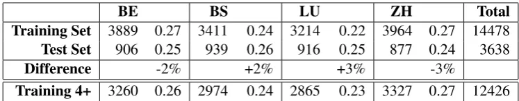
BE BS LU ZH Total Training Set 3889 0.27 3411 0.24 3214 0.22 3964 0.27 14478 Test Set 906 0.25 939 0.26 916 0.25 877 0.24 3638

Difference -2% +2% +3% -3%

Training 4+ 3260 0.26 2974 0.24 2865 0.23 3327 0.27 12426

Table 1: Distribution of classes in the training and test sets of the GDI task. Row “Training 4+” shows the effect of removing sentences with less than 4 tokens on the training set composition.

Tokens 1 2 3 4 5 6 7 8 9 10+

Training 360 731 961 1244 1416 1491 1428 1317 1125 4405

Rel. 2% 5% 7% 9% 10% 10% 10% 9% 8% 30%

Test 495 530 465 450 368 320 1010

Rel. 14% 15% 13% 12% 10% 9% 28%

Table 2: Distribution of numbers of tokens per utterance in the training and test sets of the GDI task.

focus on experimenting with CRFs and character-sequence neural network classifiers. Zhang et al. (2015) achieve competitive results on character-level document classification tasks with Convo-lutional Neural Networks (CNNs). Word-level RNNs have been applied to a variety of text clas-sification tasks (Carrier and Cho, 2014). Xiao and Cho (2016) present an efficient character-level RNN document classifier.

3 Data and Methodology

In this section, we first describe the training and test data sets. Second, we detail the methods that we apply in our runs as well as report the results of post-submission experiments using RNNs. 3.1 Properties of the Data

As Table 1 shows, the GDI training data set has roughly balanced classes (a maximum of±3 per-centage points away from a uniform distribution). The official test set is slightly better balanced (a maximum of ±1 percentage points away from a uniform distribution). However, the data sets do not have the same minority/majority classes.

Another noticeable difference between the training and test data is the presence of short utter-ances. The training set has 2,052 utterances (14%) which consist of only one, two or three words. This contrasts with the test set, whose utterances contain four or more words. Predicting the dialect of a short utterance is much harder than predicting the dialect of a long one. We systematically drop very short utterances from the training data in or-der to compensate for the differences between the

data sets3_{and to reduce the noise.}

The data only contain lowercase characters. Due to the variability in the dialects, many of the 14,065 word types appear only once (9,372), twice (2,032), or three times (929). This extreme Zipfian distribution makes it hard to build reliable statist-ics for prediction.

3.2 Our Methods

All our methods except the RNNs use character n-gram features derived from separate words. 3.2.1 Run 1: Na¨ıve Bayes

Run 1 is our baseline, which has proven hard to beat. For the final submission, we drop from the training set short noisy utterances and substitute character combinations for characters with com-plex diacritics (e.g. “¨u2” for “`¨u”) and single char-acters for the common digraph “ch” and trigraph “sch”. All one-character words are dropped. We represent each utterance with a bag of character n-grams, ranging from bigrams to six-grams. This set-up produces the highest average validation

ac-3_{This violates the default assumption in machine learning}

Figure 1: Per-dialect distribution of numbers of tokens and characters per utterance in the training set.

curacy among competing configurations (e.g. dif-fering in n-gram ranges). We use thescikit-learn

machine learning library (Pedregosa et al., 2011) to implement the entire pipeline. We fit a Na¨ıve Bayes classifier with add-one smoothing.

3.2.2 Run 2: CRF

For Run 2, we usewapiti(Lavergne et al., 2010), an efficient off-the-shelf linear-chain CRF se-quence classifier (Sutton and McCallum, 2012). Each word of an utterance is treated as a tagged item in a sequence and the utterance classification task is cast as a sequence classification of all items. For instance, the utterance “jaa ich han ja” with sequence label ZH is turned into a verticalized format corresponding to “jaa/ZH ich/ZH han/ZH ja/ZH”.

The motivation behind this approach is that a single word is often ambiguous, however, we know a priori by the definition of the task that all words in an utterance must have the same class. Therefore, we rely on the machinery of CRFs to adjust the weights of the word features in the ex-ponential model during training in such a way that sequences get optimally and homogeneously clas-sified. Indeed, the predicted sequence of classific-ation tags within one utterance is always consist-ent, and we take the class of the first word as the class of the whole utterance.

The features for the CRF are built from indi-vidual words. We experimented with different re-placement rules for the diacritics, but in the end just applied two phonetically motivated replace-ments (“sch” and “ch”) before feature extraction.

We use 4 types of features for the representation of a token:

WD The word form using our two replacements.

PS Concatenations of the prefix and suffix of each word (from 1 to 3 characters depending on the length of the word).

NG Character n-grams (from 1 to 6 characters). Before extracting the n-grams, we prefix each word with an “A” and suffix it with a “Z” in order to distinguish n-grams at word bound-aries from n-grams within a word.

CV Word shapes selecting or mapping character classes for consonants and vowels. Specific-ally, feature types V and C contain all vow-els and consonants of a word in the order of appearance. Feature types Cs and Vs contain the sets of all consonants and vowels, respect-ively. Feature types VV and CC contain the word shape where either all vowels or all con-sonants get masked with a “C” or a “V”. Fea-ture type CCVV masks all characters with a “C” or a “V”.

b Each word also has a so-called bigram output feature that encodes the transition probabil-ity of class labels. This ensures that the sys-tem learns to predict sequences with only ho-mogeneous class labels. The unigram output feature “u”, which encodes the global distri-bution of class labels, was not useful, how-ever.

CRF tools like wapiti allow each feature to be used as evidence only for the class of the current token (feature prefix “u:”) or the class of the preceding and/or current token (feature prefix “*:”).4 _{For the}

GDI task, we only use “u:” features. Thus, for a word like “vernoo” (en: heard), the following features are extracted:

Length in words Replaced with Example 10≥l >15 a) First 3/4 of words,

and b) last 3/4 “a a de a der annere wand sis schwiizer welo”annere wand sis”, b) “de a der annere wand sis schwiizer welo”⇒a) “a a de a der l≥15 a) First 2/3 of words,

b) last 2/3, and c) 1/3 in the middle

“aber das h¨and d¨ann d schuurnalischten am prozss zum biischpil isch d¨a saz wider choo”⇒a) “aber das h¨and d¨ann d schuurn-alischten am proz¨ass zum biischpil”, b) “schuurnschuurn-alischten am proz¨ass zum biischpil isch d¨a saz wider choo”, c) “h¨and d¨ann d schuurnalischten am proz¨ass zum biischpil isch d¨a saz” Table 3: Data augmentation rules.

WD=vernoo b u:PS=vo u:PS=veoo

u:NG=Av u:NG=Ave u:NG=v u:NG=ve

u:NG=ver u:NG=e u:NG=er u:NG=ern

u:NG=r u:NG=rn u:NG=rno u:NG=n u:NG=no u:NG=noo u:NG=o u:NG=oo u:NG=ooZ u:NG=o u:NG=oZ u:V=eoo u:C=vrn u:Cs=nrv

u:Vs=eo u:VV=vVrnVV u:CC=CeCCoo

u:CCVV=CVCCVV.

The CV word shape features add about one per-centage point in accuracy.

A typical training fold (90% of the training data) results in about 540,000 different feature candidates. After thirty five training epochs us-ing the Elastic Net regularization (Zou and Hastie, 2005), around 90,000 features are still active.

The only hyper-parameter that we need to ad-just is the maximal number of training epochs of the L-BFGS optimizer (Liu and Nocedal, 1989). A maximum of thirty five training epochs guarantees optimal performance. We use a development set of 10% of the training set to control for overfitting and finding a reasonable number of epochs. Still, we find no clear and smooth convergence. Chan-ging the default parameters for the Elastic Net reg-ularization or any other hyper-parameter of wap-iti does not result in systematic and consistent im-provements.

3.2.3 Run 3: Ensemble of Na¨ıve Bayes, CRF, and linear SVM

Run 3 is a majority-vote ensemble system built from the results of Run 1, Run 2, and predictions generated from a linear SVM over the same fea-ture model as for Run 1. Whenever all classifiers disagree with one another, the ensemble falls back to the prediction by the Run 1 system. We used

scikit-learn’s implementation of linear SVM train-able with the Stochastic Gradient Descent optim-ization algorithm and searched for the value of the regularization parameter with the highest average cross-validation accuracy.

3.2.4 Experiments with LSTMs

We have invested a considerable amount of ef-fort in RNN models. We implement particularly simple Long Short-Term Memory (LSTM) net-works (Hochreiter and Schmidhuber, 1997): with and without an initial character embedding layer, with a recurrent layer, and a softmax output layer. Like in the other runs, we experiment with single character and character group replacements. We fix the size of the character embedding layer to two thirds the input size, which therefore varies from model to model as a result of character replace-ments (twenty five or twenty nine units). The size of the LSTM layer is fixed to ninety hidden units. The softmax layer takes as input the values of the LSTM hidden units at the final character. All the models are rather small, with the leanest models having 41,760 parameters and the largest having 48,600 parameters. Adding a character embedding layer results in a 9% reduction in model paramet-ers, on average. The reduction in the number of character types shrinks the model by another 4%, and the replacement of common di- and trigraphs shortens input sequences and further speeds up training. We discarded the idea of using bidirec-tional LSTMs (Graves and Schmidhuber, 2005): They are slower to train (the number of model parameters roughly doubles), which has been the main bottleneck for us since we have intended to experiment with multiple model set-ups.

com-Run 1 Run 2 Run 3

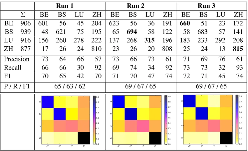
Σ BE BS LU ZH BE BS LU ZH BE BS LU ZH

BE 906 601 56 45 204 623 56 36 191 660 51 23 172

BS 939 48 621 75 195 65 694 58 122 58 683 57 141

LU 916 156 260 278 222 137 268 315 196 183 233 292 208

ZH 877 17 26 24 810 23 26 20 808 25 24 13 815

Precision 73 64 66 57 73 66 73 61 71 69 76 61

Recall 66 66 30 92 69 74 34 92 73 73 32 93

F1 70 65 42 70 71 70 47 74 72 71 45 74

P / R / F1 65 / 63 / 62 69 / 67 / 65 69 / 67 / 65

Table 4: Confusion matrices and result breakdown for our official GDI runs. Rows are true labels, columns are predicted labels.

Run Accuracy F1 (macro) F1 (weighted) Baseline 25.80

1 63.50 61.65 61.56 2 67.07 65.38 65.31

3 67.34 65.34 65.27

Table 5: Official results for the GDI task. The baseline predicts the majority class. For all classes, F1 (micro) is the same as accuracy.

pletely (in this case, one-word and two-word ut-terances). As a result of this data augmentation, the training data for the internal system evaluation have grown by almost a quarter (from 11,726 to 15,340 utterances).

All neural-network implementation is done us-ing high-level structures of the keras neural net-works library (Chollet, 2015). For training the models, we use the Root Mean Square Propaga-tion (RMSProp) algorithm (Tieleman and Hinton, 2012), a variant of Stochastic Gradient Descent, with default hyper-parameters suggested by the library. We use Dropout (Srivastava et al., 2014) for regularization. We train for at least 100 epochs and at most 300 epochs.

4 Results

4.1 Official Results

Table 5 shows the official results of our submitted runs. Run 3 has the best accuracy among our runs, but is slightly worse on the macro-averaged F1 score and the weighted F1 score (see Zampieri et al. (2017) for further information on the evaluation metrics). The performance in absolute numbers is much lower than expected from cross-validation. 4.2 Internal Evaluation

Cross-validation results Internal evaluation set results Run Accuracy F1 (macro) F1 (weighted) Accuracy F1 (macro) F1 (weighted)

1 85.10 (0.82) 84.99 (0.82) 85.10 (0.82) 85.43 85.36 85.44

2 83.96 (0.68) 83.87 (0.70) 83.93 (0.69) 85.01 85.02 85.01

3 85.70 (0.59) 85.57 (0.60) 85.68 (0.60) 85.50 85.42 85.50 SVM 82.46 (0.59) 82.36 (0.64) 82.43 (0.61) 82.39 82.36 82.39

LSTM - - - 83.49 83.30 83.46

Table 6: System comparison: Results for ten-fold stratified cross-validation and performance on an internal evaluation set. Cross validation results: We report mean scores across the folds and indicate standard deviations in parentheses. The SVM is a model from the ensemble of Run 3.

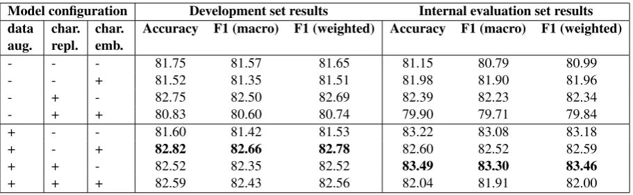
Model configuration Development set results Internal evaluation set results data

aug. char.repl. char.emb. Accuracy F1 (macro) F1 (weighted) Accuracy F1 (macro) F1 (weighted)

- - - 81.75 81.57 81.65 81.15 80.79 80.99

- - + 81.52 81.35 81.51 81.98 81.90 81.96

- + - 82.75 82.50 82.69 82.39 82.23 82.34

- + + 80.83 80.60 80.74 79.90 79.71 79.84

+ - - 81.60 81.42 81.53 83.22 83.08 83.18

+ - + 82.82 82.66 82.78 82.60 82.52 82.59

+ + - 82.52 82.35 82.52 83.49 83.30 83.46

+ + + 82.59 82.43 82.56 82.04 81.91 82.00

Table 7: Comparison of RNN sequence classifiers.

5 Discussion

ZH clearly dominates in terms of recall in all our runs (Table 4). The recognition rates for ZH, BE, and BS are fine (around 70% F1) in our official runs. However, the F1 score for LU is much lower (around 45%) due to severe recall problems. The numbers show that the recognition of LU suffers from more frequent predictions in favor of ZH and BS. This behavior fits the empirical distribution of the classes from the training set (short sentences removed) as shown in Table 1 where 27% of all sequences are ZH, but only 23% LU. As the prob-lem may also lie in the data, it would be interesting to see whether all the systems participating in the shared task exhibit this bias.

The results on the official test data (Table 5) are unexpectedly lower than our cross-validation estimates from the training data (67% accuracy instead of about 88% with short sequences re-moved). Clearly, the training and test sets have not been consistently sampled from the same dis-tribution.

The Na¨ıve Bayes classifier of Run 1 has been exceptionally strong on same-domain data. Inter-estingly, it suffers worse compared to other sys-tems from differently sampled data.

According to our observation during training, CRFs seem to run a bit into convergence problems. Therefore, one might try to systematically build more varying models (for instance, by bootstrap sampling and randomly selected subsets of extrac-ted features) in order to have a broader ensemble system. Another line of work that we could not complete due to time restrictions is the integra-tion of a word predicintegra-tion model into the CRF system based on character-level CNNs (Xiao and Cho, 2016). Our expectation would be that con-volution filters might be better at learning relevant character-level representations for estimating the label probability for a given word.

and +0.3%, respectively). On the other hand, mod-els with a character embedding layer and/or char-acter replacements are faster to reach higher ac-curacy levels. Just like with other models, short utterances pose the largest difficulty, and perform-ance goes up with utterperform-ance length. Overall, using slow-to-train neural models on this task has not paid off: Blazingly fast linear classifiers achieve very strong results, and so time is better spent on looking for good features.

6 Conclusion

We show that a character n-gram-based Na¨ıve Bayes approach gives a very strong baseline for the classification of transcribed Swiss German dia-lects, especially when test and training sets are drawn from the same distribution. The CRF-based approach works better for the official test set (ranked third by weighted F1 score among all the submitted GDI runs). The official test set is clearly sampled differently from the training set. Given a rather large performance difference of 4.5% between the Na¨ıve Bayes and the CRF, we suspect that the CRF-based approach has general-ized better than the Na¨ıve Bayes. In terms of ac-curacy, an ensemble approach using Na¨ıve Bayes, CRF, and linear SVM gives the best results of our runs and ranks second among all GDI runs. 7 Acknowledgement

We would like to thank three anonymous review-ers for their helpful comments. Peter Makarov is supported by European Research Council Grant No. 338875.

References

Pierre Luc Carrier and Kyunghyun Cho. 2014. LSTM networks for sentiment analysis. Deep Learning Tu-torials.

Franc¸ois Chollet. 2015. Keras. https://github.

com/fchollet/keras.

Eugen Dieth. 1986. Schwyzert¨utschi Dial¨akts-chrift: Dieth-Schreibung. Lebendige Mundart. Sauerl¨ander, Aarau etc. 2. Aufl. / bearb. und hrsg. von Christian Schmid-Cadalbert (1. Aufl. 1938). Alex Graves and J¨urgen Schmidhuber. 2005.

Framewise phoneme classification with bidirec-tional LSTM and other neural network architectures. Neural Networks.

Sepp Hochreiter and J¨urgen Schmidhuber. 1997. Long short-term memory.Neural computation.

J. Huang, A. Smola, A. Gretton, K. Borgwardt, and B. Schoelkopf. 2007. Correcting sample selection bias by unlabeled data. In B. Schoelkopf, J. Platt, and T. Hoffman, editors, Advances in Neural In-formation Processing Systems 19, pages 601–608. MIT Press, Cambridge, MA.

Jing Jiang and ChengXiang Zhai. 2007. Instance weighting for domain adaptation in NLP. In Pro-ceedings of the 45th Annual Meeting of the Associ-ation of ComputAssoci-ational Linguistics, pages 264–271. Association for Computational Linguistics.

Thomas Lavergne, Olivier Capp´e, and Franc¸ois Yvon. 2010. Practical very large scale CRFs. In Proceed-ings the 48th Annual Meeting of the Association for Computational Linguistics (ACL). Association for Computational Linguistics.

D. C. Liu and J. Nocedal. 1989. On the limited memory BFGS method for large scale optimization. Math. Program.

Shervin Malmasi, Marcos Zampieri, Nikola Ljubeˇsi´c, Preslav Nakov, Ahmed Ali, and J¨org Tiedemann. 2016. Discriminating between similar languages and arabic dialect identification: A report on the third dsl shared task. In Proceedings of the 3rd Workshop on Language Technology for Closely Re-lated Languages, Varieties and Dialects (VarDial), Osaka, Japan.

F. Pedregosa, G. Varoquaux, A. Gramfort, V. Michel, B. Thirion, O. Grisel, M. Blondel, P. Pretten-hofer, R. Weiss, V. Dubourg, J. Vanderplas, A. Pas-sos, D. Cournapeau, M. Brucher, M. Perrot, and E. Duchesnay. 2011. Scikit-learn: Machine learn-ing in Python. Journal of Machine Learning Re-search.

Tanja Samardzic, Yves Scherrer, and Elvira Glaser. 2016. ArchiMob – A corpus of spoken Swiss German. In Proceedings of the Language Re-sources and Evaluation (LREC), pages 4061–4066, Portoroz, Slovenia).

Yves Scherrer and Owen Rambow. 2010. Word-based dialect identification with georeferenced rules. In Proceedings of the 2010 Conference on Empirical Methods in Natural Language Processing. Associ-ation for ComputAssoci-ational Linguistics.

Fabrizio Sebastiani. 2002. Machine learning in auto-mated text categorization. ACM computing surveys (CSUR).

Nitish Srivastava, Geoffrey E Hinton, Alex Krizhevsky, Ilya Sutskever, and Ruslan Salakhutdinov. 2014. Dropout: a simple way to prevent neural networks from overfitting. Journal of Machine Learning Re-search.

Tijmen Tieleman and Geoffrey Hinton. 2012. Lecture 6.5-rmsprop: Divide the gradient by a running aver-age of its recent magnitude.

Yijun Xiao and Kyunghyun Cho. 2016. Efficient character-level document classification by combin-ing convolution and recurrent layers. CoRR. Marcos Zampieri, Shervin Malmasi, Nikola Ljubeˇsi´c,

Preslav Nakov, Ahmed Ali, J¨org Tiedemann, Yves Scherrer, and No¨emi Aepli. 2017. Findings of the VarDial Evaluation Campaign 2017. InProceedings of the Fourth Workshop on NLP for Similar Lan-guages, Varieties and Dialects (VarDial), Valencia, Spain.

Xiang Zhang, Junbo Zhao, and Yann LeCun. 2015. Character-level convolutional networks for text clas-sification. In Advances in neural information pro-cessing systems.