Neural Transition based Syntactic Linearization

431

Neural Transition-based Syntactic Linearization

Linfeng Song1, Yue Zhang2 and Daniel Gildea1

1_{Department of Computer Science, University of Rochester, Rochester, NY 14627} 2_{School of Engineering, Westlake University, China}

Abstract

The task of linearization is to find a gram-matical order given a set of words. Tradi-tional models use statistical methods. Syn-tactic linearization systems, which gen-erate a sentence along with its syntactic tree, have shown state-of-the-art perfor-mance. Recent work shows that a multi-layer LSTM language model outperforms competitive statistical syntactic lineariza-tion systems without using syntax. In this paper, we study neural syntactic lineariza-tion, building a transition-based syntactic linearizer leveraging a feed forward neural network, observing significantly better re-sults compared to LSTM language models on this task.

1 Introduction

Linearization is the task of finding the grammat-ical order for a given set of words. Syntactic linearization systems generate output sentences along with their syntactic trees. Depending on how much syntactic information is available dur-ing decoddur-ing, recent work on syntactic lineariza-tion can be classified into abstract word ordering

(Wan et al.,2009;Zhang et al., 2012;de Gispert

et al., 2014), where no syntactic information is

available during decoding, full tree linearization

(He et al.,2009;Bohnet et al.,2010;Song et al.,

2014), where full tree information is available, and partial tree linearization (Zhang,2013), where par-tial syntactic information is given as input. Lin-earization has been adapted to tasks such as ma-chine translation (Zhang et al., 2014), and is po-tentially helpful for many NLG applications, such as cooking recipe generation (Kiddon et al.,2016), dialogue response generation (Wen et al., 2015), and question generation (Serban et al.,2016).

Previous work (Wan et al., 2009; Liu et al.,

2015) has shown that jointly predicting the syn-tactic tree and the surface string gives better re-sults by allowing syntactic information to guide statistical linearization. On the other hand, most such methods employ statistical models with dis-criminative features. Recently, Schmaltz et al.

(2016) report new state-of-the-art results by lever-aging a neural language modelwithoutusing syn-tactic information. In their experiments, the neu-ral language model, which is less sparse and cap-tures long-range dependencies, outperforms previ-ous discrete syntactic systems.

A research question that naturally arises from this result is whether syntactic information is help-ful for a neural linearization system. We em-pirically answer this question by comparing a neural transition-based syntactic linearizer with the neural language model of Schmaltz et al.

(2016). Following Liu et al. (2015), our lin-earizer works incrementally given a set of words, using a stack to store partially built dependency trees, and a set to maintain unordered incoming words. At each step, it either shiftsa word onto the stack, or reduces the top two partial trees on the stack. We leverage a feed forward neural net-work, which takes stack features as input and pre-dicts the next action (such as SHIFT, LEFTARC

and RIGHTARC). Hence our method can be re-garded as an extension of the parser ofChen and

Manning(2014), adding word ordering

function-alities.

and the gap can go up to 11 BLEU points by in-tegrating the LSTM language model as features. The integrated system also outperforms the LSTM language model by 1 BLEU point using beam search, which shows that syntactic information is useful for a neural linearization system.

2 Related work

Previous work (White, 2005; White and

Rajku-mar,2009;Zhang and Clark,2011;Zhang,2013)

on syntactic linearization uses best-first search, which adopts a priority queue to store partial hy-potheses and a chart to store input words. At each step, it pops the highest-scored hypothesis from the priority queue, expanding it by combination with the words in the chart, before finally putting all new hypotheses back into the priority queue. As the search space is huge, a timeout threshold is set, beyond which the search terminates and the current best hypothesis is taken as the result.

Liu et al.(2015) adapt the transition-based

de-pendency parsing algorithm for the linearization task by allowing the transition-based system to shift any word in the given set, rather than the first word in the buffer as in dependency parsing. Their results show much lower search times and higher performance compared to Zhang (2013). Following this line, Liu and Zhang (2015) fur-ther improve the performance by incorporating an n-gram language model. Our work takes the transition-based framework, but is different in two main aspects: first, we train a feed-forward neu-ral network for making decisions, while they all use perceptron-like models. Second, we investi-gate a light version of the system, which only uses word features, while previous works all rely on POS tags and arc labels, limiting their usability on low-resource domains and languages.

Schmaltz et al.(2016) are the first to adopt

neu-ral networks on this task, while only usingsurface features. To our knowledge, we are the first to leverage both neural networks and syntactic fea-tures. The contrast between our method and the method of Chen and Manning(2014) is reminis-cent of the contrast between the method of Liu

et al.(2015) and the dependency parser ofZhang

and Nivre (2011). Comparing with the

depen-dency parsing task, which assumes that POS tags are available as input, the search space of syntactic linearization is much larger.

Recent work (Zhang, 2013;Song et al., 2014;

Liu et al., 2015; Liu and Zhang, 2015) on

syn-tactic linearization uses dependency grammar. We follow this line of works. On the other hand, lin-earization with other syntactic grammars, such as context free grammar (de Gispert et al.,2014) and combinatory categorial grammar (White and

Ra-jkumar, 2009; Zhang and Clark, 2011), has also

been studied.

3 Task

Given an input bag-of-wordsx={x1, x2, ..., xn}, the goal is to output the correct permutation y, which recovers the original sentence, from the set of all possible permutationsY. A linearizer can be seen as a scoring functionf overY, which is trained to output its highest scoring permutation ˆ

y = argmaxy0_∈Yf(x, y0) as close as possible to the correct permutationy.

3.1 Baseline: an LSTM language model

The LSTM language model of Schmaltz et al.

(2016) is similar to the medium LSTM setup of

Zaremba et al.(2014). It contains two LSTM

lay-ers, each of which has 650 hidden units and is followed by a dropout layer during training. The multi-layer LSTM language model can be repre-sented as:

ht,i,ct,i = LSTM(ht,i−1,ht−1,i,ct−1,i) (1)

p(wt,j|wt−1, ..., w1) =

exp(v|_jht,I)

P

j0exp(v|_j0ht,I)

, (2)

whereht,iandct,iare the output and cell memory

of thei-th layer at stept, respectively,ht,0 =xtis

the input of the network at stept,Iis the number of layers, wt,j represents outputtingwj att step,

vjis the embedding ofwj, and the LSTM function

is defined as:



  

i f o g



  

=



  

σ σ σ

tanh



  

W4n,2n

ht,i−1 ht−1,i

(3)

ct,i =f ct−1,i+ig (4)

ht,i =otanh(ct,i), (5)

where σ is the sigmoid function, W4n,2n is the

weights of LSTM cells, andis the element-wise product operator.

<bos> I

I love love NLP

NLP <eos>

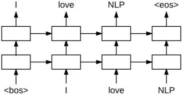
Figure 1: Linearization procedure of the baseline.

{“NLP”,“love”,“I”}as input. At each step, it takes the output word from the previous step as input and predicts the current word, which is chosen from the remaining input bag-of-words rather than from the entire vocabulary. Therefore it takes n

steps to linearize a input consisting ofnwords.

4 Neural transition-based syntactic

linearization

Transition-based syntactic linearization can be considered as an extension to transition-based de-pendency parsing (Liu et al.,2015), with the main difference being that the word order is not given in the input, so that any word can be shifted at each step. This leads to a much larger search space. In addition, under our setting,extradependency rela-tions or POS on input words are not available.

The output building process is modeled as a state-transition process. As shown in Figure 2, each states is defined as (σ, ρ, A), where σ is a stack that maintains a partial derivation,ρis an un-orderedset of incoming input words andAis the set of dependency relations that have been built. Initially, the stackσis empty, while the setρ con-tains all the input words, and the set of depen-dency relations A is empty. At the end, the set

ρis empty, whileAcontains all dependency rela-tions for the predicted dependency tree. At a cer-tain state, a SHIFTaction chooses one word from

the set ρand pushes it onto the stack σ, a LEFT -ARC action makes a new arc{j ← i} from the stack’s top two items (iandj), while a RIGHTARC

action makes a new arc{j →i}fromiandj. Us-ing these possible actions, the unordered word set

{“NLP0”,“love1”,“I2”} is linearized as shown in Table1, and the result is “I2 ←love1→NLP0”.1

1_{For a clearer introduction to our state-transition process,}

we omit the POS-pactions, which are introduced in Section

4.2. In our implementation, each SHIFT-wis followed by exact one POS-paction.

Figure 2: Deduction system of transition-based syntactic linearization

step action σ ρ A

init [] (1 2 3) ∅

0 Shift-I [1] (2 3)

1 Shift-love [1 2] (3)

2 Shift-NLP [1 2 3] ()

3 RArc-dobj [1 2] () A∪ {2→3}

4 LArc-nsubj [2] () A∪ {1←2}

5 End [] () A

Table 1: Transition-based syntactic linearization for ordering{“NLP3”,“love2”,“I1”}, whereRArc andLArc are the abbreviations for RightArc and LeftArc, respectively. More details on actions are in Section4.2.

4.1 Model

To predict the next transition action for a given state, our linearizer makes use of a feed-forward neural network to score the actions as shown in Figure3. The network takes a set of word, POS tag, and arc label features from the stack as in-put and outin-puts the probability distribution of the next actions. In particular, we represent each word as ad-dimensional vectorew_i ∈ Rdusing a word

embedding matrix isEw ∈ _Rd×Nw_{, whereNw is}

the vocabulary size. Similarly each POS tag and arc label are also mapped to ad-dimensional vec-tor, whereet_j,el_k ∈ _Rd_{are the representations of}

thej-th POS tag andk-th arc label, respectively. The embedding matrices of POS tags and arc la-bels are Et ∈ _Rd×Nt _{and E}l _∈

Rd×Nl, where NtandNlcorrespond to the number of POS tags

and arc labels, respectively. We choose a set of feature words, POS tags, and arc labels from the stack context, using their embeddings as input to our neural network. Next, we map the input layer to the hidden layer via:

....

... ...

Words POS tags arc labels

Input Layer Hidden

Layer Output

Layer

....

Figure 3: Neural syntactic linearization model

where xw, xt, and xl are the concatenated fea-ture word embeddings, POS tag embeddings, and arc label embeddings, respectively,Ww₁,Wt₁, and W₁l are the corresponding weight matrices, b1 is the bias term andg()is the activation function of the hidden layer. The word, POS tag and arc label features are described in Section4.3.

Finally, the hidden vectorhis mapped to an out-put layer, which uses a softmax activation function for modeling multi-class action probabilities:

p(a|s, θ) = softmax(W2h), (7)

wherep(a|s, θ)represents the probability distribu-tion of the next acdistribu-tion. There is no bias term in this layer and the model parameterW2 can also be seen as the embedding matrix of all actions.

4.2 Actions

We use 5 types of actions:

• SHIFT-wpushes a wordwonto the stack.

• POS-p assigns a POS tag p to the newly

shifted word.

• LEFTARC-lpops the top two itemsiandjoff

stack and pushes{j←−l i}onto the stack.

• RIGHTARC-lpops the top two itemsiandj

off stack and pushes{j−→l i}onto the stack.

• ENDends the decoding procedure.

Given a set ofnwords as input, the linearizer takes 3nsteps to synthesize the sentence. The number of actions is large, making it computationally in-efficient to do softmax over all actions. Here for each set of wordsSwe only consider all possible actions for linearizing the set, which constraints SHIFT-wi to all words in the set.

(1) S1.w;S1.t;S2.w;S2.t;S3.w;S3.t;

(2)

i= 1,2

lc1(Si).w;lc1(Si).t;lc1(Si).l;

lc2(Si).w;lc2(Si).t;lc2(Si).l;

rc1(Si).w;rc1(Si).t;rc1(Si).l;

rc2(Si).w;rc2(Si).t;rc2(Si).l;

(3)

i= 1,2

lc1(lc1(Si)).w;lc1(lc1(Si)).t;

lc1(lc1(Si)).l;rc1(rc1(Si)).w;

rc1(rc1(Si)).t;rc1(rc1(Si)).l;

Table 2: Feature templates, whereSi denotes the ith item on the stack,w,tandldenotes the word, POS tag and arc label, respectively.

4.3 Features

The feature templates our model uses are shown in Table2. We pick (1) the words and POS tags of the top 3 items on the stack, (2) the words, POS tags, and arc labels of the first and the second left-most / rightleft-most children of the top 2 items on the stack and (3) the words, POS tags and arc labels of the leftmost of leftmost / rightmost of rightmost children of the top two items on the stack. Under certain states, some features may not exist, and we use special tokens NULLw, NULLtand NULLlto represent non-existent word, POS tag, and arc la-bel features, respectively. Our feature templates are similar to that of Chen and Manning (2014), except that we do not leverage features from the set, because the words inside the set are unordered.

4.4 The light version

We also consider a light version of our linearizer that only leverages words and unlabeled depen-dency relations. Similar to Section 4.1, the sys-tem also uses a feed-forward neural network with 1 hidden layer, but only takes word features as in-put. It uses 4 types of actions: SHIFT-w, LEFT -ARC, RIGHTARC, and END. All actions are same

as described in Section4.2, except that LEFTARC

and RIGHTARCare not associated with arc labels. Given a set ofnwords as input, the system takes 2nsteps to synthesize the sentence, which is faster and less vulnerable to error propagation.

5 Integrating an LSTM language model

Our model can be integrated with the baseline multi-layer LSTM language model. Existing work

(Zhang et al., 2012; Liu and Zhang, 2015) has

the integration: (1) joint decoding by interpolat-ing the conditional probabilities and (2) feature-level integration by taking the output vector (hI)

of the LSTM language model as features to the linearizer.

5.1 Joint decoding

To perform joint decoding, the conditional action probability distributions of both models given the current state are interpolated, and the best action under the interpolated probability distribution is chosen, before both systems advancing to a new state using the action. The interpolated conditional probability is:

p(a|s_i, hi;θ1, θ2) = logp(a|si;θ1)

+αlogp(a|h_i;θ2), (8)

wheresiandθ1are the state and parameters of the linearizer, hi andθ2 are the state and parameters of the LSTM language model, andαis the inter-polation hyper parameter.

The action spaces of the two systems are dif-ferent because the actions of the LSTM language model correspond only to the shift actions of the linearizer. To match the probability distributions, we expand the distribution of the LSTM language model as shown in Equation 9, where wa is the

associated word of a shift action a. Generally, the probabilities of non-shift actions are 1.0, and those of shift actions are from the LSTM language model with respect towa:

p(a|hi;θ2) =

(

p(wa|hi;θ2), ifais shift

1.0, otherwise (9)

We do not normalize the interpolated probability distribution, because our experiments show that normalization only gives around 0.3 BLEU score gains, while significantly decreasing the speed. When a shift action is chosen, both systems ad-vance to a new state; otherwise only the linearizer advances to a new state.

5.2 Feature level integration

To take the output of an LSTM language model as a feature in our model, we first train the LSTM lan-guage model independently. During the training of our model, we takehI, the output of the top LSTM layer after consuming all words on the stack, as a feature in the input layer of Figure3, before finally advancing both the linearizer and the LSTM lan-guage model using the predicted action. This is

analogous to adding a separately-trained n-gram language model as a feature to a discriminative linearizer (Liu and Zhang,2015). Compared with joint decoding (Section 5.1), p(a|s_i, hi;θ1, θ2) is calculated by one model, and thus there is no need to tune the hyper-parameter α. The state update remains the same: the language model advances to a new state only when a shift action is taken.

6 Training

Following Chen and Manning (2014), we set the training objective as maximizing the log-likelihood of each successive action conditioned on the dependency tree, which can be gold or au-tomatically parsed. To train our linearizer, we first generate training examples{(si, ti)}mi=1 from the training sentences and their gold parse trees, wheresi is a state, andti ∈ T is the correspond-ing oracle transition. We use the “arc standard” oracle (Nivre,2008), which always prefers SHIFT

over LEFTARC. The final training objective is to minimize the cross-entropy loss, plus an L2-regularization term:

L(θ) =−X i

logpti+ λ

2kθk 2_,

where θ represents all the trainable parameters: W1,b1,W2,Ew,Et,El. A slight variation is that the softmax probabilities are computed only among the feasible transitions in practice. As de-scribed in Section 4.2, for an input set of words, the feasible transitions are: SHIFT-w, wherewis a word in the set, POS-pfor all POS tags, LEFTARC

-land RIGHTARC-lfor all arc labels, and END.

To train a linearizer that takes an LSTM lan-guage model as features, we first train the LSTM language model on the same training data, then train the linearizer with the parameters of the LSTM language model unchanged.

7 Experiments

7.1 Setup

We follow previous work and conduct experiments on the Penn Treebank, using Wall Street Journal sections 2-21 for training, 22 for development and 23 for final testing. Gold-standard dependency trees are derived from bracketed sentences in the treebank using Penn2Malt.2 In order to study the influence of parsing accuracy of the training data,

System BEAMSIZE=1 BEAMSIZE=10 BEAMSIZE=64 BEAMSIZE=512

BLEU Time BLEU Time BLEU Time BLEU Time

LSTM 14.01 6m26s 26.83 13m 33.05 54m41s 37.08 405m10s

SYN 20.97 11m39s 27.72 26m40s 30.01 113m19s 31.12 891m39s

SYN+LSTM 21.17 18m15s 30.43 37m15s 34.35 157m16s 36.84 1058m

SYN×LSTM 24.91 18m12s 32.75 37m12s 35.88 156m50s 36.96 1070m

SYNl×LSTM 24.55 9m50s 32.84 23m7s 36.11 77m6s 37.99 624m39s

Table 3: Main results and decoding times.

ID #training sent #iter F1

syn90 all 30 90.28

syn85 all 1 85.38

syn79 9000 1 79.68

syn54 900 1 54.86

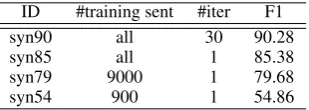
Table 4: Parsing accuracy settings, the F1 scores are measured on the training set.

we use ten-fold jackknifing to construct WSJ train-ing data with different accuracies. More specifi-cally, the data is first randomly split into ten equal-size subsets, and then each subset is automati-cally parsed with a constituent parser trained on the other subsets, before the results are finally con-verted to dependency trees using Penn2Malt. In order to obtain datasets with different parsing ac-curacies, we randomly sample a small number of sentences from each training subset and choose different training iterations, as shown in Table4. In our experiments, we use ZPar3 _{(Zhu et al.,} 2013) for automatic constituent parsing.

Our syntactic linearizer is implemented with Keras.4 We randomly initializeEw, Et, El, W1 andW2within(−0.01,0.01), and use default set-ting for other parameters. The hyper-parameters and parameters which achieve the best perfor-mance on the development set are chosen for final evaluation. Our vocabulary comes from SENNA5, which has 130,000 words. The activation func-tions tanhand softmax are added on top of the hidden and output layers, respectively. We use Adagrad (Duchi et al.,2011) with an initial learn-ing rate of 0.01, regularization parameter λ = 10−8, and dropout rate 0.3 for training. The in-terpolation coefficient α for joint decoding is set 0.4. During decoding, simple pruning methods are applied, such as a constraint that POS-pactions al-ways follow SHIFT-wactions.

We evaluate our linearizer (SYN) and its vari-ances, where the subscript “l” denotes the light

3

https://github.com/frcchang/zpar 4

https://keras.io/

5_{http://ronan.collobert.com/senna/}

version, “+LSTM” represents joint decoding with an LSTM language model, and “×LSTM” repre-sents taking an LSTM language model as features in our model. We compare results with the cur-rent state-of-the-art: an LSTM (LSTM) language model fromSchmaltz et al.(2016), which is sim-ilar in size and architecture to the medium LSTM setup of Zaremba et al.(2014). None of the sys-tems use future cost heuristic. All experiments are conducted using Tesla K20Xm.

7.2 Tuning

We show some development results in this sec-tion. First, using the cube activation function

(Chen and Manning,2014) does not yield a good

performance on our task. We tried other activa-tions includingLinear,tanhandReLU(Nair and

Hinton, 2010), and tanh gives the best results.

In addition, we tried pretrained embeddings from SENNA, which does not yield better results com-pared to random initialization. Further, dropout rates from0.3to0.8give good training results. Fi-nally, we tried different values from0.1to1.0for the interpolation coefficientα, finding that values between0.3 and0.7 give the best performances, while values larger than 1.5 yield poor perfor-mances.

7.3 Main results

The main results on the test set are shown in Ta-ble 3. Compared with previous work, our lin-earizers achieve the best results under all beam sizes, especially under the greedy search scenario (BEAMSIZE=1), where SYN and SYN×LSTM

outperform the baseline of LSTM by 7 and 11 BLEU points, respectively. This demonstrates that syntactic information is extremely important when beam size is small. In addition, our syntac-tic systems are still better than the baseline under very large beam sizes (such as, BEAMSIZE=512),

System sentences

LSTM-512 the bush administration , known as 31 , 1992 , earlier this year said it would extend voluntary restraint agreements steel quotas until march .

SYNl×LSTM-512 earlier this year , the bush administration said it would extend steel agreements until march 31 , 1992 , known as voluntary restraint quotas .

REF the bush administration earlier this year said it would extend steel quotas , known as voluntary re-straint agreements , until march 31 , 1992 .

LSTM-512 shearson lehman hutton inc. said , however , that it is “ going to set back with the customers , ” because of friday ’s plunge , president of jeffrey b. lane concern “ reinforces volatility relations . SYNl×LSTM-512 however , jeffrey b. lane , president of shearson lehman hutton inc. , said that friday ’s plunge is “

going to set back with customers because it reinforces the volatility of “ concern , ” relations . REF however , jeffrey b. lane , president of shearson lehman hutton inc. , said that friday ’s plunge is “

going to set back ” relations with customers , “ because it reinforces the concern of volatility . LSTM-512 the debate between the stock and futures markets is prepared for wall street will cause another

situa-tion about whether de-linkage crash undoubtedly properly renewed friday .

SYNl×LSTM-512 the wall street futures markets undoubtedly will cause renewed debate about whether the stock situa-tion is properly prepared for an other crash between friday and de-linkage .

REF the de-linkage between the stock and futures markets friday will undoubtedly cause renewed debate about whether wall street is prope rly prepared for another crash situation .

Table 5: Output samples.

The results are consistent with (Ma et al., 2014) in that both increasing beam size and using richer features are solutions for error propagation.

SYN×LSTM is better than SYN+LSTM. In fact, SYN×LSTM can be considered as

interpo-lation with α being automatically calculated un-der different states. Finally, SYNl×LSTM is

bet-ter than SYN×LSTM except under greedy search,

showing that word-to-word dependency features may be sufficient for this task.

As for the decoding times, SYN_l×LSTM shows a moderate time growth along increas-ing beam size, which is roughly 1.5 times slower than LSTM. In addition, SYN+LSTM and SYN×LSTM are the slowest for each beam size

(roughly 3 times slower than LSTM), because of the large number of features they use and the large number of decoding steps they take. SYNis

roughly 2 times slower than LSTM.

Previous work, such asSchmaltz et al. (2016), adopts future cost and the information of base noun phrase (BNP) and shows further improve-ment on performance. However, these are highly task specific. Future cost is based on the assump-tion that all words are available at the beginning, which is not true for other tasks. On the other hand, our model does not rely on this assumption, thus can be better applicable on other tasks. BNPs are the phrases that correspond to leaf NP nodes in constituent trees. Assuming BNPs being available is not practical either.

10 15 20 25 30 35 40 45 50

sentence length 0.1

0.2 0.3 0.4 0.5 0.6 0.7 0.8

BLEU

Synl×LSTM-512

Synl×LSTM-1

LSTM-512 LSTM-1

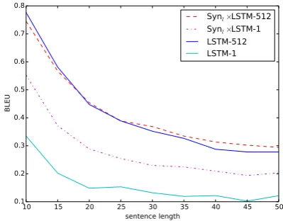
Figure 4: Performance on different lengths.

7.4 Influence of sentence length

We show the performances on different sentence lengths in Figure4. The results are from LSTM and SYNl×LSTM using beam size 1 and 512.

Sentences belonging to the same length range (such as 1–10 or 11–15) are grouped together, and corpus BLEU is calculated on each group. First of all, SYN_l×LSTM-1 is significantly bet-ter than LSTM-1 on all sentence lengths, explain-ing the usefulness of syntactic features. In ad-dition, SYN_l×LSTM-512 is notably better than LSTM-512 on sentences that are longer than 25, and the difference is even larger on sentences that have more than 35 words. This is an evidence that SYNl×LSTM is better at modeling long-distance

dependencies. On the other hand, LSTM-512 is better than SYNl×LSTM-512 on short sentences

Data SYN×LSTM SYNl×LSTM

Gold 36.03 36.41

syn90 35.91 36.31

syn85 35.84 36.22

syn79 35.40 35.96

syn54 33.32 34.98

Table 6: Results of various parsing accuracy.

good at modeling relatively shorter dependencies without syntactic guidance, while SYNl×LSTM,

which takes more steps for synthesizing the same sentence, suffers from error propagation. Overall, this figure can be regarded as empirical evidence that syntactic systems are better choices for gener-ating long sentences (Wan et al.,2009;Zhang and

Clark,2011), while surface systems may be better

choices for generating short sentences.

Table5shows some linearization results of long sentences from LSTM and SYNl×LSTM using

beam size 512. The outputs of SYNl×LSTM are

notably more grammatical than those of LSTM. For example, in the last group, the output of SYNl×LSTM means “the market will cause

an-other debate about whether the situation now is prepared for another crash”, while the output of LSTM is obviously less fluent, especially for the parts “... markets is prepared for wall street will cause ...” and “... crash undoubtedly properly re-newed ..”.

In addition, LSTM makes locally grammati-cal outputs, while suffering more mistakes in the global level. Taking the second group as an exam-ple, LSTM generates grammatical phrases, such as “going to set back with the customers” and “be-cause of friday ’s plunge”, while misplacing “pres-ident of”, which should be in the very front of the sentence. On the other hand, SYNl×LSTM

can capture patterns such as “president of some inc.” and “someone, president of someplace said” to make the right choices. Finally, SYNl×LSTM

can makes grammatical sentences with different meanings. For example in the first group, the re-sult of SYNl×LSTM means “the bush

adminis-tration will extend the steel agreement”, while the true meaning is “the bush administration will ex-tend the steel quotas”. For syntactic linearization, such semantic variation is tolerable.

7.5 Results with auto-parsed data

There is no syntactically annotated data in many domains. As a result, performing syntactic lin-earization in these domains requires automatically

Actions Top similar actions

S-wednesday S-tuesday S-friday S-thursday S-monday S-huge S-strong S-serious S-good S-large S-taxes S-bills S-expenses S-loans S-payments S-secretary S-department S-officials S-director S-largely S-partly S-primarily S-mostly S-entirely

Table 7: Top similar actions for shift actions

600 400 200 0 200 400 600

400 200 0 200 400

P-PRP$

P-VBG P-FW

P-VBN

P-POS P-''

P-VBP P-WDT

P-JJ P-WP

P-VBZ P-DT

P-#

P-RP

P-$

P-NN

P-VBD P-,

P-. P-TO

P-PRP P-RB

P--LRB-P-:

P-NNS P-NNP

P-``

P-WRB P-CC

P-LS P-PDT

P-RBS

P-RBR P-CD

P-EX

P-IN P-WP$

P-MD

P-NNPS P--RRB-P-JJS

P-JJR P-SYM

P-VB

P-UH

noun verb adjective adverb punctuation misc

Figure 5: t-SNE visualization of POS embeddings

parsed training data, which may affect the per-formance of our syntactic linearizer. We study this effect by training both SYN×LSTM and SYNl×LSTM with automatically parsed training

data of different parsing accuracies, and show the results, which are generated with beamsize 64 on the devset, in Table6. Generally, a higher parsing accuracy can lead to a better linearization result for both systems. It conforms to the intuition that syn-tactic quality affects the fluency of surface texts. On the other hand, the influence is not large, the BLEU scores of SYNl×LSTM and SYN×LSTM

drop by 1.5 and 2.8 BLEU points, respectively, as the parsing accuracy decreases from gold to 54%. Both observations are consistent with that of Liu

and Zhang(2015) for discrete syntactic

lineariza-tion. Finally, SYN_l×LSTM shows less BLEU score decreases than SYN×LSTM. The reason is

that SYNl×LSTM only takes word features, and

is less vulnerable to parsing accuracy decrease.

7.6 Embedding similarity

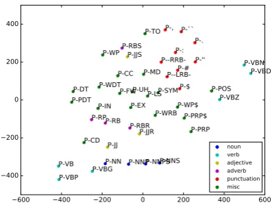
One main advantage of neural systems is that they use vectorized features, which are less sparse than discriminative features. TakingW2as the embed-ding matrix of actions, we calculate the top similar actions for the SHIFT-wactions by cosine distance

and show examples in Table 7. In addition, Fig-ure5presents the t-SNE visualization (Maaten and

actions. Generally, the embeddings of similar ac-tions are closer than these of other acac-tions. From both results, we can see that our model learns rea-sonable embeddings from the Penn Treebank, a small-scale corpus, which shows the effectiveness of our system from another perspective.

8 Conclusion

We studied neural transition-based syntactic lin-earization, which combines the advantages of both neural networks and syntactic information. In ad-dition, we compared two ways of integrating a neural language model into our system. Experi-mental results show that our system achieves im-proved results comparing with a state-of-the-art multi-layer LSTM language model. To our knowl-edge, we are the first to investigate neural syntactic linearization.

In the future work, we will investigate LSTM on this task. In particular, an LSTM decoder, tak-ing features form the already-built subtrees as part of its inputs, is taken to model the sequences of shift-reduce actions. Another possible direction is creating complete graphs with their nodes be-ing the input words, before encodbe-ing them with self-attention networks (Vaswani et al., 2017) or graph neural networks (Kipf and Welling, 2016;

Beck et al.,2018;Zhang et al.,2018;Song et al.,

2018). This approach can be better at capturing word-to-word dependencies than simply summing word embeddings up.

References

Daniel Beck, Gholamreza Haffari, and Trevor Cohn. 2018. Graph-to-sequence learning using gated graph neural networks. InProceedings of the 56th Annual Meeting of the Association for Computa-tional Linguistics (ACL-18).

Bernd Bohnet, Leo Wanner, Simon Mill, and Alicia Burga. 2010. Broad coverage multilingual deep sen-tence generation with a stochastic multi-level real-izer. InProceedings of the 23rd International Con-ference on Computational Linguistics (COLING-10). Beijing, China, pages 98–106.

Danqi Chen and Christopher Manning. 2014. A fast and accurate dependency parser using neural net-works. In Conference on Empirical Methods in Natural Language Processing (EMNLP-14). Doha, Qatar, pages 740–750.

Adri`a de Gispert, Marcus Tomalin, and Bill Byrne. 2014. Word ordering with phrase-based grammars.

InProceedings of the 14th Conference of the Euro-pean Chapter of the ACL (EACL-14). Gothenburg, Sweden, pages 259–268.

John Duchi, Elad Hazan, and Yoram Singer. 2011. Adaptive subgradient methods for online learning and stochastic optimization. Journal of Machine Learning Research12(Jul):2121–2159.

Wei He, Haifeng Wang, Yuqing Guo, and Ting Liu. 2009. Dependency based chinese sentence real-ization. In Proceedings of the 47th Annual Meet-ing of the Association for Computational LMeet-inguistics (ACL-09). Suntec, Singapore, pages 809–816.

Chlo´e Kiddon, Luke Zettlemoyer, and Yejin Choi. 2016. Globally coherent text generation with neu-ral checklist models. In Conference on Empirical Methods in Natural Language Processing (EMNLP-16). Austin, Texas, pages 329–339.

Thomas N Kipf and Max Welling. 2016. Semi-supervised classification with graph convolutional networks. arXiv preprint arXiv:1609.02907.

Jiangming Liu and Yue Zhang. 2015. An empirical comparison between n-gram and syntactic language models for word ordering. In Conference on Em-pirical Methods in Natural Language Processing (EMNLP-15). Lisbon, Portugal, pages 369–378.

Yijia Liu, Yue Zhang, Wanxiang Che, and Bing Qin. 2015. Transition-based syntactic linearization. In Conference on Empirical Methods in Natural Lan-guage Processing (EMNLP-15). Denver, Colorado, pages 113–122.

Ji Ma, Yue Zhang, and Jingbo Zhu. 2014. Punctuation processing for projective dependency parsing. In Proceedings of the 52nd Annual Meeting of the As-sociation for Computational Linguistics (ACL-14). Baltimore, Maryland, pages 791–796.

Laurens van der Maaten and Geoffrey Hinton. 2008. Visualizing data using t-sne. Journal of Machine Learning Research9(Nov):2579–2605.

Vinod Nair and Geoffrey E Hinton. 2010. Rectified linear units improve restricted Boltzmann machines. InProceedings of the 27th international conference on machine learning (ICML-10). pages 807–814.

Joakim Nivre. 2008. Algorithms for deterministic in-cremental dependency parsing. Computational Lin-guistics34(4):513–553.

Kishore Papineni, Salim Roukos, Todd Ward, and Wei-Jing Zhu. 2002. Bleu: a method for automatic eval-uation of machine translation. In Proceedings of the 40th Annual Conference of the Association for Computational Linguistics (ACL-02). Philadelphia, Pennsylvania, USA, pages 311–318.

Language Processing (EMNLP-16). Austin, Texas, pages 2319–2324.

Iulian Vlad Serban, Alberto Garc´ıa-Dur´an, Caglar Gulcehre, Sungjin Ahn, Sarath Chandar, Aaron Courville, and Yoshua Bengio. 2016. Generating factoid questions with recurrent neural networks: The 30m factoid question-answer corpus. In Pro-ceedings of the 54th Annual Meeting of the As-sociation for Computational Linguistics (ACL-16). Berlin, Germany, pages 588–598.

Linfeng Song, Yue Zhang, Kai Song, and Qun Liu. 2014. Joint morphological generation and syntactic linearization. InProceedings of the National Con-ference on Artificial Intelligence (AAAI-14). pages 1522–1528.

Linfeng Song, Yue Zhang, Zhiguo Wang, and Daniel Gildea. 2018. A graph-to-sequence model for amr-to-text generation. In Proceedings of the 56th An-nual Meeting of the Association for Computational Linguistics (ACL-18).

Ashish Vaswani, Noam Shazeer, Niki Parmar, Jakob Uszkoreit, Llion Jones, Aidan N Gomez, Łukasz Kaiser, and Illia Polosukhin. 2017. Attention is all you need. InAdvances in Neural Information Pro-cessing Systems. pages 5998–6008.

Stephen Wan, Mark Dras, Robert Dale, and C´ecile Paris. 2009. Improving grammaticality in statisti-cal sentence generation: Introducing a dependency spanning tree algorithm with an argument satisfac-tion model. InProceedings of the 12th Conference of the European Chapter of the ACL (EACL-09). Athens, Greece, pages 852–860.

Tsung-Hsien Wen, Milica Gasic, Nikola Mrkˇsi´c, Pei-Hao Su, David Vandyke, and Steve Young. 2015. Semantically conditioned LSTM-based natural lan-guage generation for spoken dialogue systems. In Conference on Empirical Methods in Natural Lan-guage Processing (EMNLP-15). Lisbon, Portugal, pages 1711–1721.

Michael White. 2005. Designing an extensible api for integrating language modeling and realization. In Proceedings of the ACL Workshop on Software. Ann Arbor, Michigan, pages 47–64.

Michael White and Rajakrishnan Rajkumar. 2009. Per-ceptron reranking for CCG realization. In Confer-ence on Empirical Methods in Natural Language Processing (EMNLP-09). Singapore, pages 410– 419.

Wojciech Zaremba, Ilya Sutskever, and Oriol Vinyals. 2014. Recurrent neural network regularization. arXiv preprint arXiv:1409.2329.

Yue Zhang. 2013. Partial-tree linearization: General-ized word ordering for text synthesis. In Proceed-ings of the International Joint Conference on Artifi-cial Intelligence (IJCAI-13).

Yue Zhang, Graeme Blackwood, and Stephen Clark. 2012. Syntax-based word ordering incorporating a large-scale language model. In Proceedings of the 13th Conference of the European Chapter of the ACL (EACL-12). Avignon, France, pages 736–746.

Yue Zhang and Stephen Clark. 2011. Syntax-based grammaticality improvement using CCG and guided search. InConference on Empirical Methods in Nat-ural Language Processing (EMNLP-11). Edinburgh, Scotland, UK., pages 1147–1157.

Yue Zhang, Qi Liu, and Linfeng Song. 2018. Sentence-state lstm for text representation. InProceedings of the 56th Annual Meeting of the Association for Com-putational Linguistics (ACL-18).

Yue Zhang and Joakim Nivre. 2011. Transition-based dependency parsing with rich non-local features. In Proceedings of the 49th Annual Meeting of the As-sociation for Computational Linguistics (ACL-11). Portland, Oregon, USA, pages 188–193.

Yue Zhang, Kai Song, Linfeng Song, Jingbo Zhu, and Qun Liu. 2014. Syntactic SMT using a discrim-inative text generation model. In Conference on Empirical Methods in Natural Language Processing (EMNLP-14). Doha, Qatar, pages 177–182.