Proceedings of NAACL-HLT 2018, pages 2081–2091
EMR Coding with Semi-Parametric Multi-Head Matching Networks
Anthony Rios
Department of Computer Science University of Kentucky
Lexington, KY
Ramakanth Kavuluru Division of Biomedical Informatics
University of Kentucky Lexington, KY
Abstract
Coding EMRs with diagnosis and procedure codes is an indispensable task for billing, sec-ondary data analyses, and monitoring health trends. Both speed and accuracy of coding are critical. While coding errors could lead to more patient-side financial burden and mis-interpretation of a patient’s well-being, timely coding is also needed to avoid backlogs and additional costs for the healthcare facility. In this paper, we present a new neural network ar-chitecture that combines ideas from few-shot learning matching networks, multi-label loss functions, and convolutional neural networks for text classification to significantly outper-form other state-of-the-art models. Our eval-uations are conducted using a well known de-identified EMR dataset (MIMIC) with a vari-ety of multi-label performance measures.
1 Introduction
Electronic medical record (EMR) coding is the process of extracting diagnosis and procedure codes from the digital record (the EMR) pertain-ing to a patient’s visit. The digital record is mostly composed of multiple textual narratives (e.g., dis-charge summaries, pathology reports, progress notes) authored by healthcare professionals, typ-ically doctors, nurses, and lab technicians. Hos-pitals heavily invest in training and retaining pro-fessional EMR coders to manually annotate all pa-tient visits by reviewing EMRs. Proprietary com-mercial software tools often termed as computer-assisted coding (CAC) systems are already in use in many healthcare facilities and were found to be helpful in increasing medical coder productiv-ity (Dougherty et al.,2013). Thus progress in au-tomated EMR coding methods is expected to di-rectly impact real world operations.
In the US, the diagnosis and procedure codes used in EMR coding are from the
Interna-tional Classification of Diseases (ICD) terminol-ogy (specifically the ICD-10-CM variant) as re-quired by the Health Insurance Portability and Accountability Act (HIPPA). ICD codes facili-tate billing activities, retrospective epidemiologi-cal studies, and also enable researchers to aggre-gate health statistics and monitor health trends. To code EMRs effectively, medical coders are ex-pected to have thorough knowledge of ICD-10-CM and follow a complex set of guidelines to code EMRs. For example, if a coder accidentally uses the code “heart failure” (ICD-10-CM code I50) in-stead of “acute systolic (congestive) heart failure” (ICD-10-CM code I50.21), then the patient may be charged substantially more1causing significant
unfair burden. Therefore, it is important for coders to have better tools at their disposal to find the most appropriate codes. Additionally, if coders become more efficient, hospitals may hire fewer coders to reduce their operating costs. Thus auto-mated coding methods are expected to help with expedited coding, cost savings, and error control.
In this paper, we treat medical coding of EMR narratives as a multi-label text classification prob-lem. Multi-label classification (MLC) is a ma-chine learning task that assigns a set of labels (typically from a fixed terminology) to an in-stance. MLC is different from multi-class prob-lems, which assign a single label to each exam-ple from a set of labels. Compared to general multi-label problems, EMR coding has three dis-tinct challenges. First, with thousands of ICD codes, the label space is large and the label dis-tribution is extremely unbalanced – most codes occur very infrequently with a few codes occur-ring several orders of magnitude more than oth-ers. Second and more importantly, a patient may have a large number of diagnoses and procedures.
1https://nyti.ms/2oxrjCv
On average, coders annotate an EMR with more than 20 such codes and hence predicting the top one or two codes is not sufficient for EMR cod-ing. Third, EMR narratives may be very long (e.g., discharge summaries may have over 1000 words), which may result in a needle in a haystack situa-tion when attempting to seek evidence for particu-lar codes.
Recent advances in extreme multi-label classi-fication have proven to work well for large label spaces. Many of these methods (Yu et al.,2014; Bhatia et al.,2015;Liu et al.,2017) focus on cre-ating efficient multi-label models that can handle 104 to 106 labels. While these models perform well in large label spaces, they don’t necessarily focus on improving prediction of infrequent la-bels. Typically, they optimize for the top 1, 3, or 5 ranked labels by focusing on the P@1, P@3, and P@5 evaluation measures. The labels ranked at the top usually occur frequently in the dataset and it is not obvious how to handle infrequent labels. One solution would be to ignore the rare labels. However, when the majority of medical codes are infrequent, this solution is unsatisfactory.
While neural networks have shown great promise for text classification (Kim, 2014; Yang et al.,2016;Johnson and Zhang,2017), the label imbalances associated with EMR coding hinder their performance. Imagine if a dataset contains only one training example for every class leading toone-shot learning, a subtask offew-shot learn-ing. How can we classify a new instance? A triv-ial solution would be to use a non-parametric 1-NN (1 nearest neighbor) classifier. 1-1-NN does not require learning any label specific parameters and we only need to define features to represent our data and a distance metric. Unfortunately, defining good features and picking the best distance metric is nontrivial. Instead of manually defining the fea-ture set and distance metric, neural network train-ing procedures have been developed to learn them automatically (Koch et al., 2015). For example, matching networks (Vinyals et al.,2016) can auto-matically learn discriminative feature representa-tions and a useful distance metric. Therefore, us-ing a 1-NN prediction method, matchus-ing networks work well for infrequent labels. However, re-searchers typically evaluate matching networks on multi-class problems without label imbalance. For EMR coding with extreme label imbalance with several labels occurring thousands of times,
tra-ditional parametric neural networks (Kim, 2014) should work very well on the frequent labels. In this paper, we introduce a new variant of matching networks (Vinyals et al., 2016;Snell et al.,2017) to address the EMR coding problem. Specifically, we combine the non-parametric idea ofk-NN and
matching networks with traditional neural network text classification methods to handle both frequent and infrequent labels encountered in EMR coding. Overall, we make the following contributions in this paper:
• We propose a novel semi-parametric neural
matching network for diagnosis/procedure code prediction from EMR narratives. Our architecture employs ideas from matching networks (Vinyals et al., 2016), multiple at-tention (Lin et al., 2017), multi-label loss functions (Nam et al., 2014a), and convolu-tional neural networks (CNNs) for text clas-sification (Kim,2014) to produce a state-of-the-art EMR coding model.
• We evaluate our model on publicly available EMR datasets to ensure reproducibility and benchmarking; we also compare against prior state-of-the-art methods in EMR coding and demonstrate robustness across multiple stan-dard evaluation measures.
• We analyze and measure how each
compo-nent of our model affects the performance us-ing ablation experiments.
2 Related Work
In this section we cover recent methodologies that are either relevant to our approach and problem or form the main ingredients of our contribution.
2.1 Extreme Multi-label Classification
based on how they reduce the label space and how the projection operation is optimized. Tai and Lin (2012) use principal component analy-sis (PCA) to reduce the label space. Low-rank Em-pirical risk minimization for Multi-Label Learning (LEML) (Yu et al.,2014) jointly optimizes the la-bel space reduction and the projection processes. RobustXML (Xu et al.,2016) is similar to LEML but it treats infrequent labels as outliers and mod-els them separately.Liu et al.(2017) employ neu-ral networks for extreme multi-label problems us-ing a funnel-like architecture that reduces the la-bel vector dimensionality. Tree-based multi-lala-bel methods work by recursively splitting the feature space. These methods usually differ based on the node splitting criterion. FastXML (Prabhu and Varma, 2014) partitions the feature space using the nDCG measure as the splitting criterion. Pfas-treXML (Jain et al.,2016) improves on FastXML by using a propensity scored nDCG splitting cri-terion and re-ranking the predicted labels to opti-mize various ranking measures.
2.2 Memory Augmented Neural Networks
Memory networks (Weston et al.,2014) have ac-cess to external memory, typically consisting of information the model may use to make predic-tions. Intuitively, informative memories concern-ing a given instance are found by the memory net-work to improve its predictive power.Kamra et al. (2017) use memory networks to fix issues of catas-trophic forgetting. They show that external mem-ory can be used to learn new tasks without for-getting previous tasks. Memory networks are now applied to a wide variety of natural language pro-cessing tasks, including question answering and language modeling (Sukhbaatar et al.,2015; Bor-des et al.,2015;Miller et al.,2016).
Matching networks (Vinyals et al.,2016;Snell et al., 2017) have recently been developed for few/one-shot learning problems. We can interpret matching networks as a key-value memory net-work (Miller et al.,2016). The “keys” are training instances, while the “values” are the labels asso-ciated with each training example. Intuitively, the concept is similar to a hashmap. The model will search for the most similar training instance to find its respective “value”. Also, matching networks can be interpreted as a k-NN based model that
automatically learns an informative distance met-ric. Finally,Altae-Tran et al.(2017) used
match-ing networks for drug discovery, a problem where data is limited.
2.3 Diagnosis Code Prediction
The 2007 shared task on coding radiology re-ports (Pestian et al.,2007) was the first effort that popularized automated EMR coding. Tradition-ally, linear methods have been used for diagno-sis code prediction. Perotte et al. (2013) devel-oped a hierarchical support vector machine (SVM) model that takes advantage of the ICD-9-CM hier-archy. In our prior work, we train a linear model for every label (Rios and Kavuluru, 2013) and re-rank the labels using a learning-to-rank proce-dure (Kavuluru et al., 2015).Zhang et al.(2017) supplement the diagnosis code training data with data from PubMed (biomedical article corpus and search system) to train linear models using both the original training data and the PubMed data.
Recent advances in neural networks have also been put to use for EMR coding: Baumel et al. (2018) trained a CNN with multiple sigmoid out-puts using binary cross-entropy. Duarte et al. (2017) use hierarchical recurrent neural networks (RNNs) to annotate death reports with ICD-10 codes. Vani et al. (2017) introduced grounded RNNs for EMR coding. They found that itera-tively updating their predictions at each time step significantly improved the performance. Finally, similar to our work, memory networks (Prakash et al.,2017) have recently been used for diagnosis coding. However, we would like to note two sig-nificant differences between the memory network fromPrakash et al.(2017) and our model. First, they don’t use a matching network and their mem-ories rely on extracting information about each la-bel from Wikipedia. In contrast, our model does not use any auxiliary information. Second, they only evaluate on the 50 most frequent labels, while we evaluate on all the labels in the dataset.
3 Our Architecture
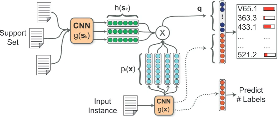
An overview of our model is shown in Figure1. Our model architecture has two main components.
1. We augment a CNN with external memory over a support setS, which consists of a small
x
CNN
g(
s
k)
V65.1
363.3
433.1
...
...
521.2
...
...
Support
Set
Input
Instance
Predict
# Labels
CNNg(x)
p
i(
x
)
h(
s
k)
[image:4.595.73.527.62.253.2]...
q
Figure 1: The matching CNN architecture. For each input instance,x, we search a support set using different representations ofxand use the similar support instances and auxiliary features to the output layer.
with similar labels. Therefore, we use the re-lated support set examples as auxiliary fea-tures. The similar instances are chosen au-tomatically by combining ideas from metric learning and neural attention. We emphasize that unlike in a traditionalk-NN setup, we do
NOT explicitly use the labels of the support set instances. The support set essentially en-riches and complements the features derived from the input instance.
2. Rather than predicting labels by thresholding, we rank them and select the topklabels
spe-cific to each instance wherekis predicted us-ing an additional output unit (termed MetaL-abeler). We train the MetaLabeler along with the classification loss using a multi-task train-ing scheme.
Before we go into more specific details of our ar-chitecture, we introduce some notation. Let X
represent the set of all training documents andx
be an instance ofX. Likewise, letSrepresent the set of support instances andsbe an instance ofS.
We letLbe the total number of unique labels. Our
full model is described in following subsections.
3.1 Convolutional Neural Networks
We use a CNN to encode each document follow-ing what is now a fairly standard approach consist-ing of an embeddconsist-ing layer, a convolution layer, a max-pooling layer, and an output layer (Collobert et al.,2011;Kim,2014). However, in our architec-ture, the CNN additionally aids in getting
interme-diate representations for the multi-head matching network component (Section3.2).
Intuitively, CNNs make use of the sequential nature of text, where a non-linear function is ap-plied to region vectors formed from vectors of words in short adjacent word sequences. Formally, we represent each document as a sequence of word vectors,[w1,w2, . . . ,wn], wherewi ∈Rd
repre-sents the vector of thei-th word in the document.
The region vectors are formed by concatenating each window ofswords,wi−s+1||. . .||wi, into a
local region vectorcj ∈Rsd. Next,cjis passed to
a non-linear function
ˆ
cj =ReLU(W cj+b),
whereW ∈Rv×sd,b∈Rv, and ReLU is a
recti-fied linear unit (Glorot et al.,2011;Nair and Hin-ton,2010). Each row ofWrepresents a
convolu-tional filter; sovis the total number of filters. After processing each successive region vec-tor, we obtain a document representation D = [ˆc1,ˆc2, . . . ,cˆn+s−1] by concatenating each cˆj
forming a matrixD ∈ Rv×(n+s−1). Each row of Dis referred to as afeature map, formed by
differ-ent convolutional filters. Unfortunately, this repre-sentation is dependent on the length of the docu-ment and we cannot pass it to an output layer. We use max-over-time pooling to create a fixed size vector
g(s) = [ˆc1max,cˆ2max, . . . ,ˆcqmax],
3.2 Multi-Head Matching Network
Using the support set and the input instance, our goal is to estimateP(y|x, S). The support setS
is chosen based on nearest neighbors and its selec-tion process is discussed in Secselec-tion 3.4. Among instances inS, our model finds informative
sup-port instances with respect toxand creates a
fea-ture vector using them. This feafea-ture vector is com-bined with the input instance to make predictions. First, each support instancesk∈Sis projected
into the support space using a simple single-layer feed forward NN as
h(g(sk)) =ReLU(Wsg(sk) +bs),
whereWs ∈ Rz×v andbs ∈ Rz. Likewise, we
project each input instancexinto the input space
using a different feed forward neural network,
pi(g(x)) =ReLU(Wiαg(x) +biα),
where Wiα ∈ Rz×v and bi
α ∈ Rz. Compared
to the support set neural network where we use only a single network, for the input instance we haveuprojection neural networks. This means we
haveuversions ofx, an idea that is similar to
self-attention (Lin et al.,2017), where the model learns multiple representations of an instance. Here each
pi(g(x))represents a single “head” or
representa-tion of the input x. Using different weight ma-trices, [W1α, . . . ,Wαu] and[b1α, . . . ,buα], we
cre-ate different representations ofx(multiple heads).
For both the input multi-heads and the support in-stance projection, we note that the same CNN is used (also indicated in Figure1) whose output is subject to the feed forward neural nets outlined thus far in this section.
Rather than searching for a single informative support instance, we search for multiple relevant support instances. For each of theuinput instance
representations, we calculate a normalized atten-tion score
Ai,k =
exp(−d(pi(g(x)), h(g(sk)))
P
sk0∈S
exp(−d(pi(g(x)), h(g(sk0)))
whereAi,krepresents the score of thek-th support
example with respect to thei-th input
representa-tionpi(g(x))and
d(xi,xj) =kxi−xjk22,
is the square of the Euclidean distance between the input and support representations.
Next, the normalized scores are aggregated into a matrix A ∈ Ru×|S|. Then, we create a feature vector
q=vec(A S) (1)
where q ∈ Ruz, vec is the matrix vectorization
operator, and S ∈ R|S|×z is the support instance
CNN feature matrix whosei-th row ish(g(si))for
i = 1, . . . ,|S|. Intuitively, multiple weighted av-erages of the support instances are created, one for each of theuinput representations. The final fea-ture vector,
h=q||g(x), (2)
is formed by concatenating the CNN representa-tion of the input instance x and the support set
feature vectorq.
Finally, the output layer for L labels involves computing
ˆ
y=P(y|x, S) =σ(Wch+bc) (3)
whereWc ∈ RL×(uz+v), bc ∈ RL, andσ is the
sigmoid function. Because we use a sigmoid acti-vation function, each label prediction (ˆyi) is in the
range from0to1.
3.3 MetaLabeler
The easiest method to convertyˆinto label predic-tions is to simply threshold each element at 0.5.
However, most large-scale multi-label problems are highly imbalanced. When training using bi-nary cross-entropy, the threshold0.5is optimized for accuracy. Therefore, our predictions will be bi-ased towards0. A simple way to fix this problem is to optimize the threshold value for each label. Unfortunately, searching for the optimal threshold of each label is computational expensive in large label spaces. Here we train a regression based out-put layer
ˆ
r =ReLU(Wrg(x) +br)
whererˆestimates the number of labelsx should be annotated with. At test time, we rank each label by its score inyˆ. Next,rˆis rounded to the nearest integer and we predict the topˆrranked labels.
3.4 Training
net-works (Nam et al.,2014b), we train using a multi-label cross-entropy loss. The loss is defined as
Lc= L
X
i=1
−yi log(ˆyi)−(1−yi) log(1−yˆi),
which sums the binary cross-entropy loss for each label. The second loss is used to train the MetaL-abeler for which we use the mean squared error
Lr=kr−ˆrk22
whereris the vector of correct numbers of labels
andˆr is our estimate. We train these two losses
using a multi-task learning paradigm (Collobert et al.,2011).
Similar to previous work with matching net-works (Vinyals et al., 2016; Snell et al., 2017), “episode” or mini-batch construction can have an impact on performance. In the multi-label setting, episode construction is non-trivial. We propose a simple strategy for choosing the support set S
which we find works well in practice. First, at the beginning of the training process we loop over all training examples and store g(x) for every train-ing instance. We will refer to this set of vectors as
T. Next, for every step of the training process (for
every mini-batchM), we searchT\Mto find the enearest neighbors (using Euclidean distance) per
instance to form our support setS. Likewise, we
adderandom examples from T \M to the
sup-port set. Therefore, our supsup-port setS contains up
to|M|e+einstances. The purpose of the random
examples is to ensure the distance metric learned during training (captured by improving represen-tations of documents as influenced by all network parameters) is robust to noisy examples.
3.5 Matching Network Interpretation
If we do not use the support set label vectors, then what is our network learning? To answer this question we directly compare the matching work formulation to our method. Matching net-works can be expressed as
ˆ
y= X
sk∈S
a(x,sk)ysk
wherea(,)is the attention/distance learned be-tween two instances, k indexes each support
in-stance, andyk is a one-hot encoded vector. a(,)
is equivalent to A1,k assuming we use a single
head. Traditional matching networks use one-hot encoded vectors because they are evaluated on multi-class problems. EMR coding is a multi-label problem. Hence, yk is a multi-hot encoded
vec-tor. Moreover, with thousands of labels, it is un-likely even for neighboring instance pairs to share many labels; this problem is not encountered in the multi-class setting. We overcome this issue by learning new output label vectors for each support set instance. Assuming a single head, our method can be re-written as
ˆ
y=σ(W1cg(x) +bc+
X
sk∈S
a(x,sk) ˜ysk), (4)
where y˜k is the learned label vector for support
instances. Next, we definey˜k, the learned support
set vectors, as
˜
ysk =W 2
ch(g(sk)) (5)
where bothW1
c andW2c are submatrices ofWc.
Using this reformulation, we can now see that our method’s main components (equations (1)-(3)) are equivalent to this more explicit matching network formulation (equations (4)–(5)). Intuitively, our method combines a traditional output layer – the first half of equation4– with a matching network where the support set label vectors are learned to better match the labels of their nearest neighbors.
4 Experiments
In this section we compare our work with prior state-of-the-art medical coding methods. In Sec-tion 4.1 we discuss the two publicly available datasets we use. Next, Section 4.2 describes the implementation details of our model. We summa-rize the various baselines and models we compare against in Section4.3. The evaluation metrics are described in Section4.4. Finally, we discuss how our method performs in Section4.5.
4.1 Datasets
# Train # Test # Labels LC AI/L MIMIC II 18822 2282 7042 36.7 118.8 MIMIC III 37016 2755 6932 13.6 80.8 Table 1: This table presents the number of training examples (# Train), the number of test examples (# Test), label cardinality (LC), and the average number of instances per label (AI/L) for the MIMIC II and MIMIC III datasets.
and the latter is the most recent version. Follow-ing prior work (Perotte et al., 2013; Vani et al., 2017), we use the free text discharge summaries in MIMIC to predict the ICD-9-CM2 codes. The
dataset statistics are shown in Table1.
For comparison purposes, we use the same MIMIC II train/test splits asPerotte et al.(2013). Specifically, we use discharge reports collected from 2001 to 2008 from the intensive care unit (ICU) of the Beth Israel Deaconess Medical Cen-ter. FollowingPerotte et al.(2013), the labels for each discharge summary are extended using the parent of each label in label set. The parents are based on the ICD-9-CM hierarchy. We use the hi-erarchical label expansion to maximize the prior work we can compare against.
The MIMIC III dataset has been extended to include health records of patients admitted to the Beth Israel Deaconess Medical Center from 2001 to 2012 and hence provides a test bed for more ad-vanced learning methods. Unfortunately, it does not have a standard train/test split to compare against prior work given we believe we are the first to look at it for this purpose. Hence, we use both MIMIC II and MIMIC III for comparison purposes. Furthermore, we do not use the hierar-chical label expansion on the MIMIC III dataset.
Before we present our results, we discuss an essential distinction between the MIMIC II and MIMIC III datasets. Particularly, we are inter-ested in the differences concerning label imbal-ance. From Table 1, we find that MIMIC III has almost twice as many examples compared to MIMIC II in the dataset. However, MIMIC II on average has more instances per label. Thus, al-though MIMIC III has more examples, each la-bel is used fewer times on average compared to
2In 2015, a federal mandate was issued that requires the
use of ICD-10 instead of ICD-9. However because of this recent change, ICD-10 training data is limited. Therefore, we use publicly available ICD-9 datasets for evaluation.
MIMIC II. The reason for this is because of how the label sets for each instance were extended us-ing the ICD-9 hierarchy in MIMIC II.
4.2 Implementation Details
Preprocessing: Each discharge summary was to-kenized using a simple regex tokenization scheme (\w\w+). Also, each word/token that occurs less than five times in the training dataset was replaced with theUNKtoken.
Model Details: For our CNN, we used convo-lution filters of size 3, 4 and 5 with 300 filters for each filter size. We used 300 dimensional skip-gram (Mikolov et al., 2013) word embed-dings pre-trained on PubMed. The Adam opti-mizer (Kingma and Ba,2015) was used for train-ing with the learntrain-ing rate 0.0001. The mini-batch size was set to 4, e – the number of
nearest neighbors per instance – was set to 16, and the number of heads (u) is set to 8. Our
code is available at: https://github.com/ bionlproc/med-match-cnn
4.3 Baseline Methods
In this paper, we focused on comparing our method to state-of-the-art methods for diagno-sis code prediction such as grounded recurrent neural networks (Vani et al., 2017) (GRNN) and multi-label CNNs (Baumel et al., 2018). We also compare against traditional binary relevance methods where independent binary classifiers (L1-regularized linear models) are trained for each label. Next, we compare against hierarchical SVM (Perotte et al.,2013), which incorporates the ICD-9-CM label hierarchy. Finally, we also re-port the results of the traditional matching network with one modification: We train the matching net-work with the multi-label loss presented in Sec-tion 3.4and threshold using the MetaLabeler de-scribed in Section3.3.
We also present two versions of our model:
Match-CNN and Match-CNN Ens. Match-CNN is the multi-head matching network introduced in Section 3. Match-CNN Ens is an ensemble that averages three Match-CNN models, each initial-ized using a different random seed.
4.4 Evaluation Metrics
MetaL-F1 AUC (PR) AUC (ROC) P@k R@k
Prec. Recall Micro Macro Micro Macro Micro Macro 8 40 8 40
Flat SVM (Perotte et al.,2013) 0.867 0.164 0.276 – – – – – – – – –
Hier. SVM (Perotte et al.,2013) 0.577 0.301 0.395 – – – – – – – – –
Logistic (Vani et al.,2017) 0.774 0.395 0.523 0.042 0.541 0.125 0.919 0.704 0.913 0.572 0.169 0.528
Attn BoW (Vani et al.,2017) 0.745 0.399 0.52 0.027 0.521 0.079 0.975 0.807 0.912 0.549 0.169 0.508
GRU-128 (Vani et al.,2017) 0.725 0.396 0.512 0.027 0.523 0.082 0.976 0.827 0.906 0.541 0.168 0.501
BiGRU-64 (Vani et al.,2017) 0.715 0.367 0.485 0.021 0.493 0.071 0.973 0.811 0.892 0.522 0.165 0.483
GRNN-128 (Vani et al.,2017) 0.753 0.472 0.58 0.052 0.587 0.126 0.976 0.815 0.93 0.592 0.172 0.548
BiGRNN-64 (Vani et al.,2017) 0.761 0.466 0.578 0.054 0.589 0.131 0.975 0.798 0.925 0.596 0.172 0.552
CNN (Baumel et al.,2018) * 0.810 0.403 0.538 0.031 0.599 0.127 0.971 0.759 0.931 0.585 0.207 0.586
Matching Network * 0.439 0.388 0.412 0.014 0.394 0.034 0.893 0.551 0.793 0.427 0.172 0.425
Match-CNN (Ours) 0.605 0.561 0.582 0.064 0.612 0.148 0.977 0.792 0.930 0.586 0.207 0.590
[image:8.595.76.525.273.367.2]Match-CNN Ens. (Ours) 0.616 0.567 0.591 0.066 0.623 0.157 0.977 0.793 0.935 0.594 0.208 0.598
Table 2: Results for the MIMIC II dataset. Models marked with * represent our custom implementations.
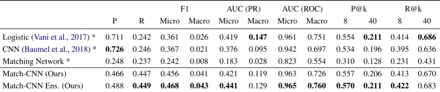
F1 AUC (PR) AUC (ROC) P@k R@k P R Micro Macro Micro Macro Micro Macro 8 40 8 40
Logistic (Vani et al.,2017) * 0.711 0.242 0.361 0.026 0.419 0.147 0.961 0.751 0.554 0.211 0.414 0.686
CNN (Baumel et al.,2018) * 0.726 0.246 0.367 0.021 0.376 0.095 0.942 0.697 0.534 0.196 0.395 0.636 Matching Network * 0.248 0.237 0.242 0.008 0.183 0.028 0.823 0.554 0.310 0.128 0.231 0.431 Match-CNN (Ours) 0.466 0.447 0.456 0.041 0.421 0.119 0.963 0.726 0.557 0.206 0.413 0.670 Match-CNN Ens. (Ours) 0.488 0.449 0.468 0.043 0.441 0.129 0.965 0.760 0.570 0.211 0.422 0.683
Table 3: Results for the MIMIC III dataset. Models marked with * represent our custom implementations.
abeler) performs when thresholding predictions. For problems with large labels spaces that suffer from significant imbalances in label distributions, the default threshold of 0.5 generally performs poorly (hence our use of MetaLabeler). To remove the thresholding effect bias, we also report differ-ent versions of the area under the precision-recall (PR) and receiver operating characteristic (ROC) curves. Finally, in a real-world setting, our system would not be expected to replace medical coders. We would expect medical coders to use our system to become more efficient in coding EMRs. There-fore, we would rank the labels based on model confidence and medical coders would choose the correct labels from the top few. To understand if our system would be useful in a real-world setting, we evaluate with precision at k(P@k) and recall
atk(R@k). Having high P@k and R@k are
crit-ical to effectively encourage the human coders to use and benefit from the system.
4.5 Results
We show experimental results on MIMIC II in Ta-ble2. Overall, our method improves on prior work across a variety of metrics. With respect to mi-cro F1, we improve upon GRNN-128 by over 1%.
Also, while macro-F1 is still low in general, we also improve macro F1 compared to state-of-the-art neural methods by more than 1%. In general, both micro and macro F1 are highly dependent on the thresholding methodology. Rather than thresh-olding at 0.5, we rank the labels and pick the topk
based on a trained regression output layer. Can we do better than using a MetaLabeler? To measure this, we look at the areas under PR/ROC curves. Regarding micro and macro PR-AUC, we improve on prior work by≈ 2.5%. This suggests that via
better thresholding, the chances of improving both micro and macro F1 are higher for Match-CNN compared to other methods. Finally, we are also interested in metrics that evaluate how this model would be used in practice. We perform compara-bly with prior work on P@k. We show strong im-provements in R@k with over a 4% improvement in R@40 compared to grounded RNNs and over 1% improvement when compared with Baumel et al.(2018). Our method also outperforms match-ing networks across every evaluation measure.
ef-F1 P@k R@k AUC (PR)
Micro Macro 8 40 8 40 Micro Macro
Match-CNN 0.456 0.041 0.557 0.206 0.413 0.670 0.421 0.119 - Matching 0.429 0.034 0.534 0.196 0.395 0.636 0.376 0.095 - MetaLabler 0.391 0.026 0.557 0.206 0.413 0.670 0.421 0.119 - Multi-Head 0.450 0.034 0.548 0.202 0.403 0.656 0.417 0.113
Table 4: Ablation results for the MIMIC III dataset.
forts. For MIMIC III also we show improve-ments in multiple evaluation metrics. Interest-ingly, our method performs much better than the standard CNN on MIMIC III, compared to the rel-ative performances of the two methods on MIMIC II. Match-CNN improves on CNN in R@40 by al-most 5% on the MIMIC III dataset. The gain in R@40 is more than the 1% improvement found on MIMIC II. We hypothesize that the improve-ments on MIMIC III are because the label imbal-ance found in MIMIC III is higher than MIMIC II. Increased label imbalances mean more labels oc-cur less often. Therefore, we believe our model works better with less training examples per label compared to the standard CNN model.
In Table 4 we analyze each component of our model using an ablation analysis on the MIMIC III dataset. First, we find that removing the matching component significantly effects our performance by reducing micro PR-AUC by almost 5%. Re-garding micro and macro F1, we also notice that the MetaLabeler heuristic substantially improves on default thresholding (0.5). Finally, we see that the multi-head matching component provides rea-sonable improvements to our model across multi-ple evaluation measures. For exammulti-ple, P@8 and P@40 decrease by around 1% when we use atten-tion with a single input representaatten-tion.
5 Conclusion
In this paper, we introduce a semi-parametric multi-head matching network with a specific ap-plication to EMR coding. We find that by combin-ing the non-parametric properties of matchcombin-ing net-works with a traditional classification output layer, we improve metrics for both frequent and infre-quent labels in the dataset. In the future, we plan to investigate three limitations of our current model.
1. We currently use a naive approach to choose the support set. We believe that improving
the support set sampling method could sub-stantially improve performance.
2. We hypothesize that a more sophisticated thresholding method could have a significant impact on the micro and macro F1 measures. As we show in Table4, MetaLabeler outper-forms naive thresholding strategies. How-ever, given our method shows non-trivial gains in PR-AUC compared to micro/macro F1, we believe better thresholding strategies are a worthy avenue to seek improvements.
3. Both the MIMIC II and MIMIC III datasets have around 7000 labels but ICD-9-CM con-tains over 16000 labels and ICD-10-CM has nearly 70,000 labels. In future work, we be-lieve significant attention should be given to zero-shot learning applied to EMR coding. To predict labels that have never occurred in the training dataset, we think it is vital to take advantage of the ICD hierarchy.Baker and Korhonen (2017) improve neural net-work training by incorporating hierarchical label information to create better weight ini-tializations. However, this does not help with respect to zero-shot learning. If we can better incorporate expert knowledge about the label space, we may be able to infer labels we have not seen before.
Acknowledgments
References
Han Altae-Tran, Bharath Ramsundar, Aneesh S Pappu, and Vijay Pande. 2017. Low data drug discov-ery with one-shot learning. ACS central science
3(4):283–293.
Simon Baker and Anna Korhonen. 2017. Initializ-ing neural networks for hierarchical multi-label text classification. BioNLP 2017pages 307–315.
Tal Baumel, Jumana Nassour-Kassis, Michael Elhadad, and Noemie Elhadad. 2018. Multi-label classifica-tion of patient notes a case study on icd code as-signment. In Proceedings of the 2018 AAAI Joint Workshop on Health Intelligence.
Kush Bhatia, Himanshu Jain, Purushottam Kar, Manik Varma, and Prateek Jain. 2015. Sparse local em-beddings for extreme multi-label classification. In
Advances in neural information processing systems. pages 730–738.
Antoine Bordes, Nicolas Usunier, Sumit Chopra, and Jason Weston. 2015. Large-scale simple question answering with memory networks. arXiv preprint arXiv:1506.02075.
Ronan Collobert, Jason Weston, L´eon Bottou, Michael Karlen, Koray Kavukcuoglu, and Pavel Kuksa. 2011. Natural language processing (almost) from scratch. Journal of Machine Learning Research
12:2493–2537.
Michelle Dougherty, Sandra Seabold, and Susan E White. 2013. Study reveals hard facts on CAC.
Journal of the American Health Information Man-agement Association84(7):54–56.
Francisco Duarte, Bruno Martins, C´atia Sousa Pinto, and M´ario J Silva. 2017. A deep learning method for icd-10 coding of free-text death certificates. In
Portuguese Conference on Artificial Intelligence. Springer, pages 137–149.
Xavier Glorot, Antoine Bordes, and Yoshua Bengio. 2011. Deep sparse rectifier networks. In Proceed-ings of the 14th International Conference on Arti-ficial Intelligence and Statistics. JMLR W&CP Vol-ume. volume 15, pages 315–323.
Himanshu Jain, Yashoteja Prabhu, and Manik Varma. 2016. Extreme multi-label loss functions for rec-ommendation, tagging, ranking & other missing la-bel applications. InProceedings of the 22nd ACM SIGKDD International Conference on Knowledge Discovery and Data Mining. ACM, pages 935–944.
Alistair EW Johnson, Tom J Pollard, Lu Shen, Li-wei H Lehman, Mengling Feng, Mohammad Ghas-semi, Benjamin Moody, Peter Szolovits, Leo An-thony Celi, and Roger G Mark. 2016. Mimic-iii, a freely accessible critical care database. Scientific data3.
Rie Johnson and Tong Zhang. 2017. Deep pyramid convolutional neural networks for text categoriza-tion. InProceedings of the 55th Annual Meeting of the Association for Computational Linguistics (Vol-ume 1: Long Papers). volume 1, pages 562–570.
Nitin Kamra, Umang Gupta, and Yan Liu. 2017. Deep generative dual memory network for continual learn-ing.arXiv preprint arXiv:1710.10368.
Ramakanth Kavuluru, Anthony Rios, and Yuan Lu. 2015. An empirical evaluation of supervised learn-ing approaches in assignlearn-ing diagnosis codes to elec-tronic medical records. Artificial intelligence in medicine65(2):155–166.
Yoon Kim. 2014. Convolutional neural networks for sentence classification. InProceedings of the 2014 Conference on Empirical Methods in Natural Lan-guage Processing (EMNLP). Association for Com-putational Linguistics, Doha, Qatar, pages 1746– 1751.
Diederik P. Kingma and Jimmy Ba. 2015. Adam: A method for stochastic optimization. In Proceed-ings of the 3rd International Conference on Learn-ing Representations (ICLR).
Gregory Koch, Richard Zemel, and Ruslan Salakhut-dinov. 2015. Siamese neural networks for one-shot image recognition. InICML Deep Learning Work-shop. volume 2.
Joon Lee, Daniel J Scott, Mauricio Villarroel, Gari D Clifford, Mohammed Saeed, and Roger G Mark. 2011. Open-access mimic-ii database for intensive care research. InEngineering in Medicine and Biol-ogy Society, EMBC, 2011 Annual International Con-ference of the IEEE. IEEE, pages 8315–8318.
Zhouhan Lin, Minwei Feng, Cicero Nogueira dos San-tos, Mo Yu, Bing Xiang, Bowen Zhou, and Yoshua Bengio. 2017. Automatic discovery and optimiza-tion of parts for image classificaoptimiza-tion. InProceedings of the International Conference on Learning Repre-sentations (ICLR).
Jingzhou Liu, Wei-Cheng Chang, Yuexin Wu, and Yiming Yang. 2017. Deep learning for extreme multi-label text classification. InProceedings of the 40th International ACM SIGIR Conference on Re-search and Development in Information Retrieval. ACM, pages 115–124.
Tomas Mikolov, Ilya Sutskever, Kai Chen, Greg S Cor-rado, and Jeff Dean. 2013. Distributed representa-tions of words and phrases and their compositional-ity. InAdvances in Neural Information Processing Systems. pages 3111–3119.
Vinod Nair and Geoffrey E Hinton. 2010. Rectified linear units improve restricted Boltzmann machines. InProceedings of the 27th International Conference on Machine Learning (ICML-10). pages 807–814.
Jinseok Nam, Jungi Kim, Eneldo Loza Menc´ıa, Iryna Gurevych, and Johannes F¨urnkranz. 2014a. Large-scale multi-label text classification - revisiting neu-ral networks. In Machine Learning and Knowl-edge Discovery in Databases - European Confer-ence, ECML PKDD 2014, Nancy, France, Septem-ber 15-19, 2014. Proceedings, Part II. pages 437– 452.
Jinseok Nam, Jungi Kim, Eneldo Loza Menc´ıa, Iryna Gurevych, and Johannes F¨urnkranz. 2014b. Large-scale multi-label text classificationrevisiting neural networks. In Machine Learning and Knowledge Discovery in Databases, Springer, pages 437–452.
Adler Perotte, Rimma Pivovarov, Karthik Natarajan, Nicole Weiskopf, Frank Wood, and No´emie El-hadad. 2013. Diagnosis code assignment: models and evaluation metrics. Journal of the American Medical Informatics Association21(2):231–237.
John P Pestian, Christopher Brew, Paweł Matykiewicz, Dj J Hovermale, Neil Johnson, K Bretonnel Cohen, and Włodzisław Duch. 2007. A shared task involv-ing multi-label classification of clinical free text. In
Proceedings of the Workshop on BioNLP 2007: Bi-ological, Translational, and Clinical Language Pro-cessing. Association for Computational Linguistics, pages 97–104.
Yashoteja Prabhu and Manik Varma. 2014. Fastxml: A fast, accurate and stable tree-classifier for extreme multi-label learning. In Proceedings of the 20th ACM SIGKDD international conference on Knowl-edge discovery and data mining. ACM, pages 263– 272.
Aaditya Prakash, Siyuan Zhao, Sadid A Hasan, Vivek V Datla, Kathy Lee, Ashequl Qadir, Joey Liu, and Oladimeji Farri. 2017. Condensed memory net-works for clinical diagnostic inferencing. InAAAI. pages 3274–3280.
Anthony Rios and Ramakanth Kavuluru. 2013. Su-pervised extraction of diagnosis codes from emrs: role of feature selection, data selection, and prob-abilistic thresholding. In Healthcare Informatics (ICHI), 2013 IEEE International Conference on. IEEE, pages 66–73.
Jake Snell, Kevin Swersky, and Richard Zemel. 2017. Prototypical networks for few-shot learning. In
I. Guyon, U. V. Luxburg, S. Bengio, H. Wallach, R. Fergus, S. Vishwanathan, and R. Garnett, editors,
Advances in Neural Information Processing Systems 30, Curran Associates, Inc., pages 4078–4088.
Sainbayar Sukhbaatar, Jason Weston, Rob Fergus, et al. 2015. End-to-end memory networks. InAdvances in neural information processing systems. pages 2440–2448.
Farbound Tai and Hsuan-Tien Lin. 2012. Multilabel classification with principal label space transforma-tion. Neural Computation24(9):2508–2542.
Grigorios Tsoumakas, Ioannis Katakis, and Ioannis P. Vlahavas. 2010. Mining multi-label data. InData Mining and Knowledge Discovery Handbook, pages 667–685.
Ankit Vani, Yacine Jernite, and David Sontag. 2017. Grounded recurrent neural networks. arXiv preprint arXiv:1705.08557.
Oriol Vinyals, Charles Blundell, Tim Lillicrap, Daan Wierstra, et al. 2016. Matching networks for one shot learning. In Advances in Neural Information Processing Systems. pages 3630–3638.
Jason Weston, Sumit Chopra, and Antoine Bor-des. 2014. Memory networks. arXiv preprint arXiv:1410.3916.
Chang Xu, Dacheng Tao, and Chao Xu. 2016. Robust extreme multi-label learning. InKDD. pages 1275– 1284.
Zichao Yang, Diyi Yang, Chris Dyer, Xiaodong He, Alex Smola, and Eduard Hovy. 2016. Hierarchi-cal attention networks for document classification. InProceedings of the 2016 Conference of the North American Chapter of the Association for Computa-tional Linguistics: Human Language Technologies. pages 1480–1489.
Hsiang-Fu Yu, Prateek Jain, Purushottam Kar, and Inderjit S. Dhillon. 2014. Large-scale multi-label learning with missing labels. InProceedings of the 31th International Conference on Machine Learn-ing, ICML 2014, BeijLearn-ing, China, 21-26 June 2014. pages 593–601.