Extracting Latent Attributes from Video Scenes Using Text as
Background Knowledge
Anh Tran, Mihai Surdeanu, Paul Cohen
University of Arizona
{trananh, msurdeanu, prcohen}@email.arizona.edu
Abstract
We explore the novel task of identify-ing latent attributes in video scenes, such as the mental states of actors, using only large text collections as background knowledge and minimal information about the videos, such as activity and actor types. We formalize the task and a measure of merit that accounts for the semantic re-latedness of mental state terms. We de-velop and test several largely unsupervised information extraction models that iden-tify the mental states of human partici-pants in video scenes. We show that these models produce complementary informa-tion and their combinainforma-tion significantly outperforms the individual models as well as other baseline methods.
1 Introduction
“Labeling a narrowly avoided vehicular manslaughter as approach(car, person) is missing something.”1 The recognition of
ac-tivities, participants, and objects in videos has advanced considerably in recent years (Li et al., 2010; Poppe, 2010; Weinland et al., 2011; Yang and Ramanan, 2011; Ng et al., 2012). However, identifying latent attributes of scenes, such as the mental states of human participants, has not been addressed. Latent attributes matter: If a video surveillance system detects one person chasing another, the response from law enforcement should be radically different if the people are happy (e.g., children playing) or afraid and angry (e.g., a person running from an assailant).
This work is licenced under a Creative Commons Attribution 4.0 International License. Page numbers and proceedings footer are added by the organizers. License details: http: //creativecommons.org/licenses/by/4.0/
1James Donlon, former manager of DARPA’s Mind’s Eye program, personal communication.
Attributes that are latent in visual representa-tions are often explicit in textual representarepresenta-tions. This suggests a novel method for inferring latent attributes: Use explicit features of videos to query text corpora, and from the resulting texts extract attributes that are latent in the videos, such as men-tal states. The contributions of this work are:
1: We formalize the novel task of latent attribute identification from video scenes, focusing on the identification of actors’ mental states. The input for the task is contextual information about the scene, such as detections about the activity (e.g., chase) and actor types (e.g., policeman or child), and the output is a distribution over mental state labels. We show that gold standard annotations for this task can be reliably generated using crowd sourcing. We define a novel evaluation measure, calledconstrained weighted similarity-alignedF1 score, that accounts for both the differences be-tween mental state distributions and the seman-tic relatedness of mental state terms (e.g., partial credit is given foriratewhen the target isangry).
2:We propose several robust and largely unsuper-vised information extraction (IE) models for iden-tifying the mental state labels of human partici-pants in a scene, given solely the activity and actor types: a lexical semantic (LS) model that extracts mental state labels that are highly similar to the context of the scene in a latent, conceptual vector space; and an information retrieval (IR) model that identifies labels commonly appearing in sentences related to the explicit scene context. We show that these models are complementary and their combi-nation performs better than either model, alone.
3: Furthermore, we show that an event-centric model that focuses on the mental state labels of the participants in the relevant event (identified us-ing syntactic patterns and coreference resolution) outperforms the above shallower models.
2 Related Work
As far as we know, the task proposed here is novel. We can, however, review work relevant to each part of the problem and our solution. Mental state inference is often formulated as a classifica-tion problem, where the goal is to predict target mental state labels based on low-level sensory in-put data. Most solutions try to learn classification models based on large amounts of training data, while some require human engineering of domain knowledge. Hidden Markov Models (HMMs) and Dynamic Bayesian Networks (DBNs) are popular representations because they can model the tem-poral evolution of mental states. For instance, the mental states of students can be inferred from un-intentional body gestures using a DBN (Abbasi et al., 2009). Likewise, an HMM can also be used to model the emotional states of humans (Liu and Wang, 2011). Some solutions combine HMMs and DBNs in a Bayesian inference framework to yield a multi-layer representation that can do real-time inference of complex mental and emotional states (El Kaliouby and Robinson, 2004; Baltru-saitis et al., 2011). Our work differs from these approaches in several ways: It is mostly unsuper-vised, multi-modal, and requires little training.
Relevant video processing technology includes object detection (e.g., (Felzenszwalb et al., 2008)), person detection, and pose detection (e.g., (Yang and Ramanan, 2011)). Many tracking algo-rithms have been developed, such as group track-ing (McKenna et al., 2000), tracktrack-ing by learn-ing appearances (Ramanan et al., 2007), and tracking in 3D space (Giebel et al., 2004; Brau et al., 2013). For human action recognition, current state-of-the-art techniques are capable of achieving near perfect performance on the com-monly used KTH Actions dataset (Schuldt et al., 2004) and high performance rates on other more challenging datasets (O’Hara and Draper, 2012; Sadanand and Corso, 2012).
To extract mental state information from texts, one might use any or all of the technologies of natural language processing, so a complete review of relevant technologies is impossible, here. Of immediate relevance is the work of de Marneffe et al. (2010), which identified the latent meaning behind scalar adjectives (e.g., which ages people have in mind when talking about “little kids”). The authors learned these meanings by extract-ing scalars, such as children’s ages, that were
commonly collocated with phrases, such as “lit-tle kids,” in web documents. Mohtarami et al. (2011) tried to infer yes/no answers from indirect yes/no question-answer pairs (IQAPs) by predict-ing the uncertainty of sentiment adjectives in in-direct answers. Their method employs antonyms, synonyms, word sense disambiguation as well as the semantic association between the sentiment adjectives that appear in the IQAP to assign a de-gree of certainty to each answer. Sokolova and La-palme (2011) further showed how to learn a model for predicting the opinions of users based on their written contents, such as reviews and product de-scriptions, on the Web. Gabbard et al. (2011) found that coreference resolution can significantly improve the recall rate of relations extraction with-out much expense to the precision rate.
Our work builds on these efforts by combining information retrieval, lexical semantics, and event extraction to extract latent scene attributes.
3 Data
For the experiments in this paper, we focus solely on videos containing chase scenes. Chases often invoke clear mental state inferences, and depend-ing on context can suggest very different mental state distributions for the actors involved.
3.1 Video Corpus
We compiled a video dataset of 26 chase videos found on the Web. Of these, five involve police officers, seven involve children, four show sports-related scenes, and twelve describe different chase scenarios involving civilian adults (two videos in-volve children playing sports). The average dura-tion of the dataset is8.8seconds with a range of [4,18]. Most videos involve a single chaser and a single chasee (a person being chased) while a few have several chasers and/or chasees.
gen-eral, we found that most responses were good and only a few incomplete submissions were rejected. In the first experiment, we asked MTurk work-ers to select the actor types and various other de-tections from a predefined list of tags. This label-ing task is a proxy for a computer vision detection system that functions at a human level of perfor-mance. Indeed, we restricted the actor type labels to a set that can be reasonably expected from auto-matic detection algorithms: person,police officer, child, and (non-human) object. For instance, po-lice officers often wear distinctive color uniforms that can be learned using the Felzenszwalb detec-tor (Felzenszwalb et al., 2008), whereas children can be reliably differentiated by their heights un-der a 3D-tracking model (Brau et al., 2013). Each video was annotated by three different workers and the union of their annotations is produced. The overall accuracy of the annotation was excel-lent. The MTurk workers correctly identified the important actors in every video.
Next, we collected a gold standard list of mental state labels for each video by asking MTurk work-ers to identify all applicable mental state adjec-tives for the actors involved. We used a text-box to allow for free-form input. Studies have shown that people of different cultures can perceive emo-tions very differently, and having forced choice options cannot always capture their true percep-tion (Gendron et al., 2014). Therefore, we did not restrict the response of the workers in any way. Workers could abstain from answering if they felt the video was too ambiguous. Each video was evaluated by ten different workers. We converted each term provided to the closest adjective form if possible. Terms with no equivalent adjective forms were left in place. On rare occasions, work-ers provided sentence descriptions despite being asked for single-word adjectives. These sentences were either removed, or collapsed into a single word if appropriate. The overall quality of the an-notations was good and generally followed com-mon intuition. Asides from the frequently used terms, we also received some colorful (yet infor-mative) descriptions, likeincredulousand vindic-tive. In general, chases involving police scenar-ios often contained violent and angry states while chases involving children received more cheerful labels. There were unexpected descriptions, such asannoyfor a playful chase between two children. Upon review of the video, we agreed that one child
did indeed look annoyed. Thus, the resulting de-scriptions were subjective, but very few were hard to rationalize. By aggregating the answers from the workers, we generated a gold standard distri-bution of mental state terms for each video.2
3.2 Text Corpus
The text corpus used for our models is the En-glish Gigaword 5th Edition corpus3, made
avail-able by the Linguistics Data Consortium and in-dexed by Lucene4. It is a comprehensive archive
of newswire text data (approximately26GB), ac-quired over several years. It is in this corpus that we expect to find mental state terms cued by con-textual information from videos.
4 Neighborhood Models
We developed several individual models based on the neighborhood paradigm, that is, the hypoth-esis that relevant mental state labels will appear “near” text cued by the visual features of a scene.
The models take as input thecontext extracted from a video scene, defined simply as a list of “ac-tivity and actor-type” tuples (e.g., (chase,police)). Multiple actor types will result in multiple tuples for a video. The actors can be either a person, a policeman, a child, or a (non-human) object. If the detections describe the actor as both a person and a child, or a person and a policeman, we auto-matically remove thepersonlabel as it is a Word-Net (Miller, 1995) hypernym of bothchildand po-liceman. For each human actor type, we further increase our coverage by retrieving the synonym set (synset) of its most frequent sense (i.e., sense #1) from WordNet. For example, a chase involv-ing a policeman would generate the followinvolv-ing tu-ples: (chase,policeman) and (chase,officer).
We call thesequery tuplesbecause they are used to query text for sentences that – if all goes well – will contain relevant mental state labels.
Given query tuples, our models use an initial seed set of160mental state adjectives to produce a single distribution over mental state labels, re-ferred to as the response distribution, for each video. The seed set is compiled from popular mental and emotional state dictionaries, includ-ing the Profile of Mood States (POMS) (McNair et al., 1971) and Plutchik’s wheel of emotion. We
2All videos and annotations are available at: http://trananh.github.io/vlsa
Source Example Mental State Labels
POMS alert, annoyed, energetic, exhausted, helpful,sad, terrified, unworthy, weary, etc. Plutchik angry, disgusted, fearful, joyful/joyous,sad, surprised, trusting, etc. Others agitated, competitive, cynical, disappointed,excited, giddy, happy, inebriated, violent, etc.
Table 1: The initial seed set contains160mental state labels, compiled from different sources like the popular Profile of Mood States dictionary and Plutchik’s wheel of emotion.
also included frequently used labels gathered from synsets found in WordNet (see Table 1 for exam-ples). Note that the gold standard annotations pro-duced by MTurk workers (Sec. 3) was not a source for this set, nor was it restricted to these terms.
4.1 Back-off Interpolation in Vector Space
Our first model uses the recurrent neural net-work language model (RNNLM) of Mikolov et al. (2013) to project both mental state labels and query tuples into a latent conceptual space. Simi-larity is then trivially computed as the cosine sim-ilarity between these vectors. In all of our experi-ments, we used a RNNLM computed over the Gi-gaword corpus with600-dimensional vectors.
For this vector space (vec) model, we separate the query tuples into different levels of back-off context. The first level includes the set of activ-ity types as singleton context tuples, e.g., (chase), while the second level includes all (activity,actor) context tuples. Hence, each query tuple will yield two different context tuples, one for each back-off level. For each context tuple with multiple terms, such as (chase,policeman), we find the vector rep-resentation for the context by aggregating the vec-tors representing the search terms:
vec(chase,policeman) = vec(chase) +
vec(policeman).
The vector representation for a singleton con-text tuple is just the vector of the single search term. We then calculate the distance of each men-tal state labelmto the normalized vector represen-tation of the context tuple by computing the cosine similarity score between the two vectors:
cos(Θm) = ||vecvec((mm))|| ||·vecvec(context tuple)(context tuple)|| .
The hypothesis here is that mental state labels that are related to the search context will have a
RNNLM vector that is closer to the context tuple vector, resulting in a high cosine similarity score. Because the number of latent dimensions is rela-tively small (when compared to vocabulary size), cosine similarity scores in this latent space tend to be close. To further separate these scores, we raise them to an exponential power:
score(m) =ecos(Θm)+1−1.
The processing of each context tuple yields160 different scores, one for each mental state label. We normalize these scores to form a single bution of scores for each context tuple. The distri-butions are then integrated into a single distribu-tion representative of the complete activity as fol-lows: (a) the distributions at each context back-off level are averaged to generate a single distribution per level – for the second level (which includes activity and actor types), it means distributions for all (activity, actor) tuples are averaged, whereas the first level only has a single distribution from the singleton activity tuple (chase); and (b) distri-butions for the different levels are linearly interpo-lated, similar to the back-off strategy of (Collins, 1997). Lete1ande2represent the weights of some mental state labelmfrom the average distribution at the first and second level, respectively. Then the interpolated distribution scoreeformis:
e=λe1+ (1−λ)e2.
Compiling the distribution scores for each m
produces the final distribution representing the ac-tivity modeled. We prune this final distribution by taking the top ranked items that make up someγ
proportion of the distribution. We delay the dis-cussion of howγ is tuned to Section 6. The final pruned distribution is normalized to produce the response distribution.
4.2 Sentence Co-occurrence with Deleted Interpolation
appear as an adjective or verb, the activity as a verb, and the actor as a noun. (Mental state adjec-tives are allowed to appear as verbs because some are often mis-tagged as verbs; e.g., agitated, deter-mined, welcoming.) We used Stanford’s CoreNLP toolkit for tokenization and POS tagging.5
Note that this probability is similar to a trigram probability in POS tagging, except the triples need not form an ordered sequence but must appear in the same sentence and under the correct POS tag. Unfortunately, we cannot always compute this tri-gram probability directly from the corpus because there might be too few instances of each trigram to compute a probability reliably. As is common, we instead estimate it as a linear interpolation of unigrams, bigrams, and trigrams. We define the maximum likelihood probabilitiesPˆ, derived from relative frequenciesf, for the unigrams, bigrams, and trigrams as follows:
ˆ
P(m) = f(Nm)
ˆ
P(m|activity) = f(fm,(activity)activity)
ˆ
P(m|activity,actor) = f(fm,(activityactivity,actor),actor)
for all mental state labelsm, activities, and actor types in our queries. N is the total number of to-kens in the corpus. The aforementioned POS re-quirement is enforced:f(m)is the number of oc-currences ofmas an adjective or verb. We define
ˆ
P = 0if the corresponding numerator and denom-inator are zero. The desired trigram probability is then estimated as:
P(m|activity,actor) = λ1Pˆ(m) +
λ2Pˆ(m|activity) + λ3Pˆ(m|activity,actor).
Asλ1+λ2+λ3= 1,P represents a probability distribution. We use the deleted interpolation algo-rithm (Brants, 2000) to estimate one set of lambda values for the model, based on all trigrams.
For each query tuple generated in a video, 160 different trigrams are computed, one for each men-tal state label in the seed set, resulting in160 con-ditional probability scores. We normalize these scores into a single distribution – the mental state distribution for that query tuple. We then combine
5http://nlp.stanford.edu/software/ corenlp.shtml.
all resulting distributions, one from each query tu-ple, and take the average to produce a single dis-tribution over mental state labels for the video. As before, we prune this distribution by taking the top-ranked items that cover a large fractionγ of total probability. The pruned distribution is renor-malized to yield the final response distribution.
4.3 Event-centric with Deleted Interpolation
Thesentmodel has two limitations. On one hand, it is too sparse: the single sentence neighborhood window is too small to reliably estimate the fre-quencies of trigrams for the probabilities of men-tal state terms. On the other hand, it may be too lenient, as it extracts all mental state mentions ap-pearing in the same sentence with the activity, or event, under consideration, regardless if they ap-ply to this event or not. We address these limita-tions next with an event-centric model (event).
Intuitively, theeventmodel focuses on the men-tal state labels of event participants. Formally, these mental state terms are extracted as follows:
1: We identify event participants (or actors). We do this by analyzing the syntactic dependencies of sentences containing the target verb (e.g., chase) to find the subject and object. In most cases, the nominal subject of the verbchaseis the chaser and the direct object is the person being chased. We implemented additional patterns to model passive voice and other exceptions. We used Stanford’s CoreNLP toolkit for syntactic dependency parsing and the downstream coreference resolution.
2: Once the phrases that point to actors are iden-tified, we identify all mentions of these actors in the entire document by traversing the coreference chains containing the phrases extracted in the pre-vious step. The sentences traversed in the chains define the neighborhood area for this model.
each neighborhood that properly contain all search terms from then-gram in the correct POS.
The event model addresses both limitations of thesentmodel: it avoids the lenient extraction of mental state labels by focusing on labels associ-ated with event participants; it addresses sparsity by considering all mentions of event participants in a document.
To understand the impact of this model, we compare it against two additional baselines. The first baseline investigates the importance of focus-ing on mental state terms associated with event participants. This model, calledcoref, implements the first two steps of the above algorithm, but in-stead of extracting only mental state terms associ-ated with event actors (last step), it considers all mentions appearing anywhere in the coreference neighborhood. That is, all unique sentences tra-versed by the relevant coreference chains are first pieced together to define a single neighborhood for a given document; then the relative joint frequen-cies ofn-grams are computed by incrementing f
once for each neighborhood that contains all terms with correct POS tags.
The second baseline analyzes the importance of coreference resolution to our problem. This model is similar tosent, with the modification that it creases the size of the neighborhood window to in-clude the immediate neighbors of target sentences that contain activity labels. We call this thewin-n model: The window around a target verb contains 2n + 1 sentences. We build the context neigh-borhood by concatenating all target sentences and their windows together for a given document. This defines a single neighborhood for each document. This contrasts with the sent model, in which the neighborhood is defined for each sentence con-taining the activity label in the document, resulting in several possible neighborhoods in a document. The joint frequency f for each n-gram – where
n > 1 – is computed similarly with the coref model: it is incremented once for each neighbor-hood that contains all the terms from the n-gram in the correct POS. Frequencies for unigrams are computed similar tosent.
As before,160different trigrams are generated for each query tuple, one for each mental state la-bel in the seed set, resulting in 160 conditional probability scores. We similarly combine these scores and generate a single pruned distribution as the response for each of the model above.
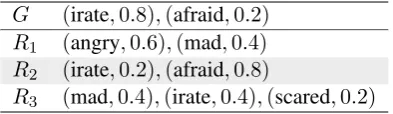
G (irate,0.8),(afraid,0.2)
R1 (angry,0.6),(mad,0.4)
R2 (irate,0.2),(afraid,0.8)
[image:6.595.319.516.62.119.2]R3 (mad,0.4),(irate,0.4),(scared,0.2) Table 2: We show an example gold standard dis-tributionGand several candidate response distri-butions to be matched against G. Here, R3 best matches the shape and meaning of G, because (irate, mad) and (afraid, scared) are close syn-onyms. R2 appears to matchGsemantically, but matches its shape poorly. R1 misses one of the mental state labels,afraid, but contains labels that are semantically close to the weightiest term inG.
4.4 Ensemble Model
We combined the results from the event and vec models to produce an ensemble model (ens) which, for a mental state labelm, returns the aver-age ofm’s scores according to the response distri-butions of the two individual models.
5 Evaluation Measures
LetRdenote the response distribution over mental state labels produced for a single video by one of the models described in the previous section, and let G denote the gold standard distribution pro-duced for the same video by MTurk workers. If
R is similar toG then our models produce simi-lar mental state terms as the workers. There are many ways to compare distributions (e.g., KL dis-tance, chi-square statistics) but these give bad re-sults when distributions are sparse. More impor-tantly, for our purposes, the measures that compare the shapes of distributions do not allow semantic comparisons at the level of distribution elements. SupposeRassigns high scores toangryandmad, only, whileGassigns a high score tohappy, only. Clearly,Ris wrong. But if insteadGhad assigned a high score toirate, only, thenRwould be more right than wrong because, at the level of the indi-vidual elements,angryandmadare similar toirate but not similar tohappy.
We describe a series of measures, starting with the familiarF1score, and discuss their applicabil-ity. To illustrate the effectiveness of each measure, we will use the examples shown in Table 2.
5.1 F1Score
andF1 = 0whenRandGshare no elements. F1 is the harmonic mean ofprecisionandrecall:
precision= |R|∩R|G|, recall= |R|G∩|G| , (1)
F1 = 2·precisionprecision+·recallrecall . (2)
The F1 score penalizes the responses in Table 3 that include semantically similar labels to those in
G, and fails to reflect the weights of the labels in
GandR.
5.2 Similarity-AlignedF1Score
Although the standardF1does not immediately fit our needs, it is a good starting point. We can in-corporate the semantic similarity of distribution el-ements by generalizing the formulas for precision and recall as follows:
precision= |R1| X
r∈R
max
g∈G σ(r, g),
recall= |G1| X
g∈G
max
r∈R σ(r, g),
(3)
whereσ ∈[0,1]is a function that yields the simi-larity between two elements. The standardF1has:
σ(r, g) =
1, ifr =g
0, otherwise ,
but clearly σ can be defined to take values pro-portional to the similarity of r and g. We can choose from a wide range of semantic similarity and relatedness measures that are based on Word-Net (Pedersen et al., 2004). The recent RNNLM of Mikolov opens the door to even more similar-ity measures based on vector space representations of words (Mikolov et al., 2013). After experi-mentations, we settled on one proposed by Hirst and St-Onge (1998). It represents two lexicalized concepts as semantically close if their WordNet synsets are connected by a path that is not too long and that “does not change direction too of-ten” (Hirst and St-Onge, 1998). We chose this metric because it has a finite range, accommodates numerous POS pairs, and works well in practice.
Given the generalized precision and recall for-mulas in Eq 3, our similarity-aligned (SA) F1 score can be computed in the usual way, as the harmonic mean of precision and recall (Eq 2).
SA-F1 is inspired by the Constrained Entity-Aligned F-Measure (CEAF) metric proposed
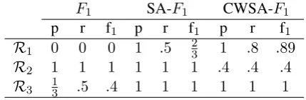
F1 SA-F1 CWSA-F1 p r f1 p r f1 p r f1
R1 0 0 0 1 .5 23 1 .8 .89
R2 1 1 1 1 1 1 .4 .4 .4
R3 13 .5 .4 1 1 1 1 1 1 Table 3: The precision (p), recall (r), and F1 (f1) scores under various evaluation models are presented for the examples from Table 2. Sup-pose that σ(irate,angry) = σ(irate,mad) =
σ(afraid,scared) = 1, with σ of any two identi-cal strings being1, andσof all other pairs are0.
by (Luo, 2005) for coreference resolution. CEAF computes an optimal one-to-one mapping between subsets of reference and system entities before it computes recall, precision and F. Similarly, SA-F1 finds optimal mappings between the labels of the two sets based onσ(this is what the max terms in Eq 3 do). Table 3 shows that SA-F1 correctly re-wards the use of synonyms. The high scores given toR2, however, indicate that it does not measure the similarity between distribution shapes.
5.3 Constrained Weighted Similarity-Aligned
F1Score
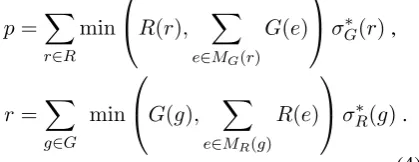
Let R(r) and G(r) be the probabilities of label
r in the R and Gdistributions, respectively. Let
σ∗
S(`)denote the best similarity score achievable
when comparing elements from set S to ` us-ing the similarity function σ. That is, σ∗
S(`) =
maxe∈Sσ(`, e). We can easily weight σS∗(`) by
the probability of `. For example, we might re-define precision asPr∈R R(r)·σ∗
G(r). However,
this would not account for the probability ofr in the gold standard distribution,G.
[image:7.595.308.523.63.133.2]mea-sure should account for an accumulated mass of synonyms. LetMS(`) denote the subset of terms
fromSthat have thebestsimilarity score to`:
MS(`) ={e|σ(`, e) =σS∗(`),∀e∈S}.
We define new forms of precision and recall as:
p=X
r∈R
min
R(r), X
e∈MG(r)
G(e) σ∗
G(r),
r=X
g∈G
min
G(g), X
e∈MR(g)
R(e) σ∗
R(g).
(4) The resulting constrained weighted similarity-aligned (CWSA) F1 score is the harmonic mean of these new precision and recall scores. Table 3 shows that CWSA-F1 yields the most intuitive evaluation of the response distributions, down-weightingR2in favor ofR3andR1.
6 Experimental Procedure
As described in Section 3, MTurk workers anno-tated 26 videos by identifying the actor types and mental state labels for each video. The actor types become query tuples of the form (activity,actor) and the mental state labels are compiled into one probability distribution over labels for each video, designatedG. The query tuples were provided to our neighborhood models (Sec. 4), which returned a response distribution over mental state labels for each video, designatedR.
We selected four videos of the 26 to calibrate the prune parameters γ and the interpolation pa-rametersλ(Sec. 4). One of these videos contains children, one has police involvement, and two con-tain adults. We asked additional MTurk workers to annotate these videos, yielding an independent set of annotations to be used solely for calibration.
The experimental question is, how well doesG
matchRfor each video? 7 Results & Discussions
[image:8.595.306.524.62.155.2]We report the average performance of our mod-els along with two additional baseline methods in Table 4. The na¨ıve baseline methodunif simply bindsR to the initial seed set of160mental state labels with uniform probability, while the stronger freq baseline uses the occurrence frequency dis-tribution of the labels from the Gigaword corpus (note that only occurrences tagged as adjectives or
F1 CWSA-F1
p r f1 p r f1
unif .107 .750 .187 .284 .289 .286
freq .107 .750 .187 .362 .352 .355
sent .194 .293 .227 .366 .376 .368
vec .226 .145 .175 .399 .392 .393
coref .264 .251 .253 .382 .461 .416
event .231 .303 .256 .446 .488 .463
ens .259 .296 .274 .488 .517 .500 Table 4: The average evaluation performance across26different chase videos are shown against 2 different baselines for all proposed models. Bold font indicates the best score in a given column.
verbs were counted). All average improvements of the ensemble model over the baseline models are significant (p <0.01). Significance tests were one-tailed and were based on nonparametric boot-strap resampling with10,000iterations.
Using the classicalF1measure, thecorefmodel scored highest on precision, while the ensemble method did best onF1. Not surprisingly, no model can top the baseline methods on recall as both baselines use the entire seed set of 160 terms. Even so, the average recall for the baselines were only.750, which means that the initial seed set did not include words that were used by the MTurk an-notators. As we’ve mentioned, the classicalF1 is misleading because it does not credit synonyms. For example, in one movie, one of our models was rewarded once for matching the label angry and penalized six times for also reporting irate, enraged, raging, upset, furious, and mad. Fre-quently, our models were penalized for using the termsscaredandafraidinstead offearful.
[image:8.595.79.289.168.249.2]Models CWSA-F1 Versuscoref p-value win-0 0.388682 −0.027512 0.0067 win-1 0.415328 −0.000866 0.4629 win-2 0.399777 −0.016417 0.0311 win-3 0.392832 −0.023362 0.0029
Table 5: The average CWSA-F1 scores for the win-nmodel with different window parameters are shown in comparison to the coref model. The coref model outperformed all tested configura-tions, though the difference is not significant for
n = 1. Thep-value based on the average differ-ences were obtained using one-tailed nonparamet-ric bootstrap resampling with10,000iterations.
Table 5 explores the effectiveness of corefer-ence resolution in expanding the neighborhood area. The coref model outperformed the simple windowing method under every tested configura-tion. However, the improvement over windowing with n = 1 is not significant. This can be ex-plained by fact that immediately neighboring sen-tences are more likely to be related. Moreover, since newswire articles tend to be short, the neigh-borhoods generated bywin-1tend to be similar to those generated by coref. In general, coref does not do worse than a simple windowing method and has the bonus advantage of providing references to the actors of interest for downstream processes.
In Table 6, we show the performance results based on the types of chase scenarios happening in the videos. The average scores under the uniform baselineunif for chase videos involving children and sporting events are lower than for police and other chases. This suggests that our seed set of 160mental state labels is biased towards the latter types of events, and is not as fit to describe chases involving children.
On average, videos involving police officers show the biggest improvement in the CWSA-F1 scores over theunif baseline (+0.2693), whereas videos involving children received the lowest gain (+0.1517). We believe this is the effect of the Gigaword text corpus, which is a comprehensive archive of newswire text, and thus is heavily bi-ased towards high-speed and violent chases in-volving the police. The Gigaword corpus is not the place to find children happily chasing each other. Similarly, sports-related chases, which are also news-worthy, have a higher gain than chil-dren’s videos on average.
Categories Unif Ensemble Gain children 0.2082 0.3599 +0.1517
police 0.3313 0.6006 +0.2693
sports 0.2318 0.4126 +0.1808 others 0.3157 0.5457 +0.2300
Table 6: The average CWSA-F1scores for the en-semble model are shown in comparison to the uni-form baseline method, categorize by video types.
8 Conclusion and Future Work
We introduced the novel task of identifying latent attributes in video scenes, specifically the men-tal states of actors in chase scenes. We showed that these attributes can be identified by using ex-plicit features of videos to query text corpora, and from the resulting texts extract attributes that are latent in the videos. We presented several largely unsupervised methods for identifying distributions of actors’ mental states in video scenes. We de-fined a similarity measure, CWSA-F1, for com-paring distributions of mental state labels that ac-counts for both semantic relatedness of the labels and their probabilities in the corresponding distri-butions. We showed that very little information from videos is needed to produce good results that significantly outperform baseline methods.
In the future, we plan to add more detection types. Additional contextual information from videos (e.g., scene locations) should help improve performance, especially on tougher videos (e.g., videos involving children chases). Moreover, we believe that the initial seed set of mental state la-bels can be learned simultaneously with the ex-traction patterns of theeventmodel using a mutual bootstrapping method, similar to that of (Riloff and Jones, 1999).
References
Abdul Rehman Abbasi, Matthew N. Dailey, Nitin V. Afzulpurkar, and Takeaki Uno. 2009. Student men-tal state inference from unintentional body gestures using dynamic Bayesian networks. Journal on Mul-timodal User Interfaces, 3(1-2):21–31, December.
Tadas Baltrusaitis, Daniel McDuff, Ntombikayise Banda, Marwa Mahmoud, Rana el Kaliouby, Peter Robinson, and Rosalind Picard. 2011. Real-time inference of mental states from facial expressions and upper body gestures. InFace and Gesture 2011, pages 909–914. IEEE, March.
Thorsten Brants. 2000. TnT: A statistical part-of-speech tagger. In Proceedings of the sixth confer-ence on Applied natural language processing, pages 224–231, Morristown, NJ, USA. Association for Computational Linguistics.
Ernesto Brau, Jinyan Guan, Kyle Simek, Luca Del Pero, Colin Reimer Dawson, and Kobus Barnard. 2013. Bayesian 3D Tracking from monocular video. InThe IEEE International Conference on Computer Vision (ICCV), December.
Michael Collins. 1997. Three generative, lexicalised models for statistical parsing. InProceedings of the 35th annual meeting on Association for Computa-tional Linguistics -, pages 16–23, Morristown, NJ, USA. Association for Computational Linguistics.
R. El Kaliouby and P. Robinson. 2004. Real-Time In-ference of Complex Mental States from Facial Ex-pressions and Head Gestures. In2004 Conference on Computer Vision and Pattern Recognition Work-shop, pages 154–154. IEEE.
Pedro Felzenszwalb, David McAllester, and Deva Ra-manan. 2008. A discriminatively trained, multi-scale, deformable part model. In2008 IEEE Confer-ence on Computer Vision and Pattern Recognition, pages 1–8. IEEE, June.
Ryan Gabbard, Marjorie Freedman, and RM Weischedel. 2011. Coreference for learn-ing to extract relations: yes, Virginia, coreference matters. InProceedings of the 49th Annual Meeting of the Association for Computational Linguistics: Human Language Technologies: short papers -Volume 2, pages 288–293.
Maria Gendron, Debi Roberson, Jacoba Marieta van der Vyver, and Lisa Feldman Barrett. 2014. Cultural relativity in perceiving emotion from vo-calizations. Psychological science, 25(4):911–20, April.
J Giebel, DM Gavrila, and C Schn¨orr. 2004. A bayesian framework for multi-cue 3d object track-ing. In Computer Vision-ECCV 2004, pages 241– 252.
Graeme Hirst and D St-Onge. 1998. Lexical chains as representations of context for the detection and cor-rection of malapropisms. In Christiane Fellbaum, editor, WordNet: An Electronic Lexical Database (Language, Speech, and Communication), pages 305–332. The MIT Press.
LJ Li, Hao Su, L Fei-Fei, and EP Xing. 2010. Ob-ject bank: A high-level image representation for scene classification & semantic feature sparsifica-tion. InAdvances in Neural Information Processing Systems.
Zhilei Liu and Shangfei Wang. 2011. Emotion recog-nition using hidden Markov models from facial tem-perature sequence. InACII’11 Proceedings of the 4th international conference on Affective computing and intelligent interaction - Volume Part II, pages 240–247.
Xiaoqiang Luo. 2005. On coreference resolution per-formance metrics. In Proceedings of the confer-ence on Human Language Technology and Empiri-cal Methods in Natural Language Processing - HLT ’05, pages 25–32, Morristown, NJ, USA. Associa-tion for ComputaAssocia-tional Linguistics.
MC De Marneffe, CD Manning, and Christopher Potts. 2010. ”Was it good? It was provocative.” Learning the meaning of scalar adjectives. InProceedings of the 48th Annual Meeting of the Association for Com-putational Linguistics, pages 167–176.
Stephen J. McKenna, Sumer Jabri, Zoran Duric, Azriel Rosenfeld, and Harry Wechsler. 2000. Tracking Groups of People. Computer Vision and Image Un-derstanding, 80(1):42–56, October.
D M McNair, M Lorr, and L F Droppleman. 1971. Profile of Mood States (POMS).
Tomas Mikolov, Kai Chen, Greg Corrado, and Jef-frey Dean. 2013. Efficient estimation of word representations in vector space. arXiv preprint arXiv:1301.3781, pages 1–12.
George A. Miller. 1995. WordNet: a lexical database for English. Communications of the ACM, 38(11):39–41, November.
Mitra Mohtarami, Hadi Amiri, Man Lan, and Chew Lim Tan. 2011. Predicting the uncertainty of sentiment adjectives in indirect answers. In Pro-ceedings of the 20th ACM international conference on Information and knowledge management - CIKM ’11, page 2485, New York, New York, USA. ACM Press.
CB Ng, YH Tay, and BM Goi. 2012. Recognizing hu-man gender in computer vision: a survey. PRICAI 2012: Trends in Artificial Intelligence, 7458:335– 346.
Ted Pedersen, S Patwardhan, and J Michelizzi. 2004. WordNet::Similarity: measuring the relatedness of concepts. In Proceedings of the Nineteenth Na-tional Conference on Artificial Intelligence (AAAI-04), pages 1024–1025, San Jose, CA.
Ronald Poppe. 2010. A survey on vision-based human action recognition. Image and Vision Computing, 28(6):976–990, June.
Deva Ramanan, David a Forsyth, and Andrew Zisser-man. 2007. Tracking people by learning their ap-pearance. IEEE transactions on pattern analysis and machine intelligence, 29(1):65–81, January. E Riloff and R Jones. 1999. Learning dictionaries for
information extraction by multi-level bootstrapping. InProceedings of the sixteenth national conference on Artificial intelligence (AAAI-1999), pages 474– 479.
S. Sadanand and J. J. Corso. 2012. Action bank: A high-level representation of activity in video. In
2012 IEEE Conference on Computer Vision and Pat-tern Recognition, pages 1234–1241. IEEE, June. C Schuldt, I Laptev, and B Caputo. 2004. Recognizing
human actions: a local SVM approach. In Proceed-ings of the 17th International Conference on Pattern Recognition, 2004. ICPR 2004., pages 32–36 Vol.3. IEEE.
M. Sokolova and G. Lapalme. 2011. Learning opin-ions in user-generated web content. Natural Lan-guage Engineering, 17(04):541–567, March. Daniel Weinland, Remi Ronfard, and Edmond Boyer.
2011. A survey of vision-based methods for action representation, segmentation and recognition. Com-puter Vision and Image Understanding, 115(2):224– 241, February.