Performance of Massive MIMO Self Backhauling for Ultra Dense Small Cell Deployments

arXiv:1806.10969v1 [cs.NI] 28 Jun 2018

Performance of Massive MIMO Self-Backhauling

for Ultra-Dense Small Cell Deployments

Andrea Bonfante

, Lorenzo Galati Giordano

, David L´opez-P´erez

, Adrian Garcia-Rodriguez

, Giovanni Geraci

,

Paolo Baracca

, M. Majid Butt

, Merim Dzaferagic

, and Nicola Marchetti

∗_{Nokia Bell Labs Ireland and}§_{Nokia Bell Labs Germany} †_{CONNECT Centre, Trinity College Dublin, Ireland}

‡_{University of Glasgow, United Kingdom}

Abstract—A key aspect of the fifth-generation wireless com-munication network will be the integration of different services and technologies to provide seamless connectivity. In this pa-per, we consider using massive multiple-input multiple-output (mMIMO) to provide backhaul links to a dense deployment of

self-backhauling (s-BH) small cells (SCs) that provide cellular access within the same spectrum resources of the backhaul. Through a comprehensive system-level simulation study, we evaluate the interplay between access and backhaul and the resulting end-to-end user rates. Moreover, we analyze the impact of different SCs deployment strategies, while varying the time resource allocation between radio access and backhaul links. We finally compare the above mMIMO-based s-BH approach to a mMIMO direct access (DA) architecture accounting for the effects of pilot reuse schemes, together with their associated overhead and contamination mitigation effects. The results show that dense SCs deployments supported by mMIMO s-BH provide significant rate improvements for cell-edge users (UEs) in ultra-dense deployments with respect to mMIMO DA, while the latter outperforms mMIMO s-BH from the median UEs’ standpoint.

Index Terms—Integrated access and backhaul, heterogeneous network, massive MIMO-based backhaul, network capacity.

I. INTRODUCTION

Fifth-generation (5G) wireless communication systems are expected to support a 1000x increase in capacity compared to existing networks [1]. Meeting this gargantuan target will require mobile network operators (MNOs) to leverage new technologies such as massive multiple-input multiple-output (mMIMO), and deploy a large number of additional small cell base stations [2], [3]. Wireless self-backhauling (s-BH), achieved through the tight integration of these two comple-mentary means, lures MNOs with the potential of achieving the desired capacity boost at a contained investment [4]. Indeed, exploiting the large number of spatial degrees-of-freedom available with mMIMO to provide sub-6 GHz in-band wireless backhauling to small cells (SCs) offers multiple advantages to MNOs: avoiding deployment of an expensive wired backhaul infrastructure, availing of more flexibility in

A. Bonfante was funded by the Irish Research Council and Nokia Ireland Ltd under the grant EPSPG/2016/106. This publication has emanated from research supported in part by a grant from Science Foundation Ireland (SFI) and is co-funded under the European Regional Development Fund under Grant Number 13/RC/2077.

the deployment of SCs, and not having to purchase additional licensed spectrum as in the case of out-of-band wireless backhauling [5].

The integration of radio access and backhauling – advocated in s-BH solutions – has been addressed by the Third Gener-ation Partnership Project (3GPP) with a list of requirements detailed in [6]. At the same time, various research efforts have tackled the problem of resource allocation and management in s-BH networks in the time and frequency domains [7], [8]. Finally, the combination of mMIMO spatial multiplexing and s-BH has been considered in [9]–[11] and also in [12]–[14], albeit for full-duplex scenarios.

In this paper, we analyze the end-to-end user equipment (UE) performance of mMIMO s-BH networks. In particular, we consider a realistic multi-cell setup where mMIMO base stations (mMIMO-BSs) provide sub-6 GHz backhauling to a plurality of half-duplex SCs overlaying the macro cellular area. We evaluate the UE data rates achieved through s-BH in two ultra-dense deployment scenarios, namely a random deployment – where SCs are uniformly distributed over a geographical area –, and an ad-hoc deployment – where SCs are purposely positioned close to UEs to achieve line-of-sight (LOS) access links. In these half-duplex systems, a s-BH approach entails sharing time-and-frequency resources between radio access and backhaul links. To the best of the authors knowledge, in this paper, we also compare for the first time the performance of the mMIMO s-BH approach and that of a direct access (DA) approach, where mMIMO-BSs are solely dedicated to serving UEs in the absence of SCs [15]. Our study provides a number of key takeaways:

• Adding morerandomly deployed SCs – where SCs are

mMIMO-BS

UE s-BH

small cell

mMIMO-BS

UE UE

mMIMO-BS

UE UE

UE

(a) Random deployment

mMIMO-BS

UE d

θ

s-BH small cell

mMIMO-BS

UE UE

mMIMO-BS

UE UE

UE

(b) Ad-hoc deployment

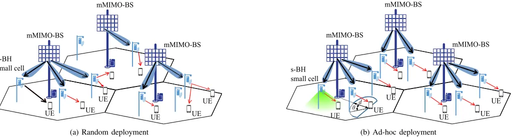
Fig. 1: Examples of two different SCs deployments considered in the paper.

radio resources and proximity, preventing the UEs to take the advantages of the SCs dense deployment.

• Addingad-hocdeployed SCs – where SCs are placed in

proximity to UEs – provides higher data rates, thanks to a high signal-to-interference-plus-noise ratio (SINR) on the access link, given by the higher proximity gains with respect to the random deployment.

• Partitioning resources between wireless access and

back-haul links is of paramount importance. Indeed, the end-to-end performance is sensitive to said partition, and optimal rates can only be achieved through a carefully designed tradeoff.

• Unlike mMIMO s-BH – where mMIMO-to-SC links

are static, and thus channel acquisition is facilitated – mMIMO DA suffers more from pilot overhead and contamination. Indeed, when compared to mMIMO DA solutions with pilot reuse 3 and reuse 1, ultra-dense SCs deployments supported by mMIMO s-BH provide rate improvements for cell-edge UEs that amount to30%and a tenfold gain, respectively. On the other hand, mMIMO DA outperforms s-BH from the median UEs’ standpoint. Notation:Capital and lower-case bold letters denote matri-ces and vectors, respectively, while [·]∗_{, [·]}T _{and [·]}H _denote

conjugate, transpose, and conjugate transpose, respectively.

II. SYSTEMMODEL

As shown in Fig. 1, we focus on the study of the down-link (DL) performance for a two-tier heterogeneous network formed by mMIMO-BSs overlaying a layer of self-backhauled SCs. The mMIMO-BSs are connected to the core network through a high-capacity wired connection, while all SCs receive backhaul traffic through mMIMO-BSs and function as access points for UEs. We consider a self-backhaul con-figuration, where mMIMO-BSs are solely dedicated for the backhaul, while SCs are solely dedicated for the access. For comparison purposes, we also consider the conventional DA approach where each mMIMO-BS directly serves the UEs.

A. Macro cell and user topologies

We denote by_Ithe set of mMIMO-BSs placed in a uniform hexagonal grid with three sectors per site. Each mMIMO-BS i, is equipped with a large number of antennasM, and serves

Li single-antenna SCs. Furthermore, we denote by Ki the number of UEs randomly and uniformly distributed over the sector’s area, and letkdenotes single-antenna UE. We assume that each UE is connected with the SC (in the s-BH approach) or with the mMIMO-BS (in the DA approach) that provides the largest reference signal received power (RSRP) [16].

B. Small cell topologies

We denote by Li the set of SCs deployed per sector and connected to the i-th mMIMO-BS that provides the largest RSRP. Each SC connectsKl UEs. Two different SCs deployments are presented in the following:

(a) Random deployment: Self-backhauled SCs are ran-domly and uniformly distributed over the mMIMO-BS geographical area as shown in Fig. 1a. This scenario is used as a baseline and follows the set of parameters specified by the 3GPP in [16] to evaluate the relay scenario.

(b) Ad-hoc deployment: Self-backhauled SCs are posi-tioned targeting nearby UE locations. This scenario is used as an example of ultra-dense network deployment. We assume the possibility to realize this target of network deployment, for example by means of drone-BSs, where the drone-BSs can reposition following the locations of UEs [17].1 As shown in Fig. 1b, we model this scenario by considering SCs deployed within a 2-D (two-dimensional) distanced of the UEs, and an angle θ measured from the straight segment that links UEs and their closest mMIMO-BS.θ is chosen uniformly at random from−π/2andπ/2. It is worth noting that even when the 2-D distance d = 0, UEs and SCs are still separated in space because the antennas are positioned at different heights. More precisely, they are assumed located at 1.5 meters and 5 meters above the ground, for the UEs and the SCs, respectively [16].

With a dense deployment of SCs, the UE SINRs are severely affected by the strong inter-cell interference among

1_{Although mentioned, the drone-BSs use-case is not the focus of this paper}

SCs. In addition, to limit the effect of the cell inter-ference, with the ad-hoc deployment, we propose to replace at the SC the isotropic antenna (Patch antenna) with a more directive antenna (Yagi antenna) pointing downwards to the ground (as shown by the green radiation cone in Fig. 1b), and therefore only illuminating the closest UEs: details about this modeling can be found in Table I.

C. Frame structure

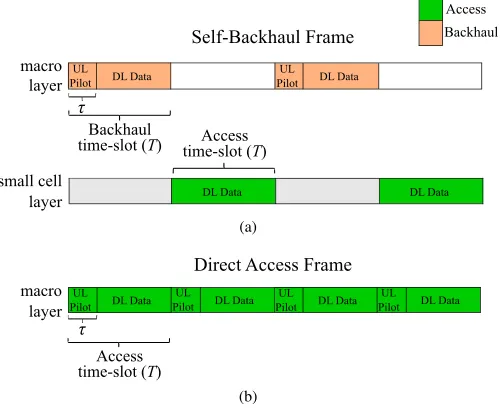
As shown in Fig. 2a, we consider the time-slot T as a single scheduling unit in the time domain, and we partition the access and backhauling resources through the parameterα∈

[0,1]. Therefore, α time-slots are allocated to the backhaul links, while1−αtime-slots are allocated to the access links. In the frequency domain, we divide the system bandwidth B into Qt resource blocks (RBs), and we allocate all the RBs to the backhaul links or the access links. We make the following assumptions in considering the partition of backhaul and access time-slots among the SCs and UEs:

• During the backhaul time-slots, all the associated SCs are

served by the mMIMO-BSi, and we use the same value ofαfor all the SCs. In this approach, the mMIMO-BSs precode the backhaul signals towards the single-antenna SCs, which are spatially multiplexed in the same time-frequency resources by allocating all the RBs in T to each SC.

• During the access time-slots, the SCs schedule their

connected UEs by using a Round Robin (RR) mechanism as frequency domain scheduler. This approach entails that each SC equally shares the system bandwidthB with its UEs.

In the Fig. 2b, it is shown the frame structure used for the DA setup, where all the time-slots are allocated to the access links. In each time slot, the mMIMO BSs precode the access signals, and the UEs are spatially multiplexed on the entire system bandwidth. Figs. 2a and 2b also show the fraction τ of the time-slots dedicated for the transmission of the pilot sequences, used to estimate the massive MIMO channel. Details about the channel training procedure will be discussed in Section III.

D. Channel model

We define as h_{il = [hil1, . . . , hilM]}T_{∈ C}M _the propaga-tion channel between the l-th single-antenna receiver (SC in the s-BH architecture and UE in the mMIMO DA) and the M antennas of thei-th mMIMO-BS. The composite channel matrix between the i-th mMIMO-BS and the devices in the i′_{-th cell is represented byH}

i,i′ = [hi1· · ·hiLi′]∈C M×Li′_. Since all the RBs are assigned to each SC, we removed the RB index qfrom the massive MIMO channel notation.

Furthermore, we define asglkq ∈Cthe input single-output (SISO) channel between the l-th SC and the k-th UE in the q-th RB. Each channel coefficient hilm =

√ βil˜hilm, andglkq=

√

βlk˜glkq accounts for both the effects of a large scale fading and a small scale fading components:

DL Data UL

Pilot DL Data

Access

Backhaul

macro layer

small cell layer

UL Pilot

Self-Backhaul Frame

τ

DL Data DL Data

Access time-slot (T) Backhaul

time-slot (T)

(a)

small cell layer macro layer

Direct Access Frame

DL Data UL

Pilot DL Data

UL

Pilot DL Data

UL Pilot DL Data

UL Pilot

Access time-slot (_T) τ

Backhaul

(b)

Fig. 2: DL frame structure for mMIMO s-BH withα= 0.5 _(Fig. 2a) and for mMIMO DA (Fig. 2b).

• The large fading components βil, βlk ∈ R+ have been modeled by using a combined LOS/Non-LOS (NLOS) path loss model, which accounts for the shadowing effect, set to be log-normal distributed with different standard deviations [16]. Because of its slow-varying characteris-tic, it does not change rapidly with time, and it can be assumed constant over the observation time-scale of the network.

• The small scale fading components ˜hilm,g˜lkq ∈ C, which results from multi-path, have been modeled as a Rician fast-fading, which rapidly changes over time and frequency. For the LOS channels, we characterize the Rician K factor with the model: K[dB] = 13−0.03r in dB, wherer is the distance between transmitter and receiver in meters [18].

Throughout the paper, we assume a composite fading (i.e. large scale fading and small scale fading together) for the SC-UE and the mMIMO-BS-UE links (in the DA approach), which changes between successive time-slots and between different RBs. Moreover, because of the static position of the SCs, we consider that the backhaul channel SC-mMIMO-BS remains constant for a periodTBH ≫T.

III. END-TO-ENDUERATES

In this section, we provide the detailed description of the operations required for the DL transmission in the mMIMO s-BH approach and in the mMIMO DA approach. We describe the channel training procedure, the mMIMO DL backhaul transmission, and the DL access transmission, which is treated separately below for both the s-BH and the mMIMO DA setups.

A. Massive MIMO channel training

associated to the same mMIMO-BS have orthogonal pilot sequences, and define the pilot code-book with the matrix Φ_{i= [φi1· · ·φiL}

i]

T

∈CLi×S

, which satisfiesΦ_iΦH i =ILi.

Here, the l-th sequence is given byφil= [φil1, . . . , φilS]T∈ CS

, and S denotes the pilot code-book length. Note that Li≤S, i.e., the maximum number of SCs or UEs served by the mMIMO-BSs in a time-slot is limited by the number of orthogonal pilot sequences. The matrix Y_{i ∈}CM×S

of pilot sequences received at thei-th mMIMO-BS can be expressed as [19]

Y_i= q

Pul

il X

i′_∈I

H_i,i′Φ_i′+N_{i, (1)}

where Pul

il is the power used by the l-th device located in the i-th sector for UL pilot transmission, and N_{i ∈} CM×S represents an additive noise, and is modeled with independent and identically distributed complex Gaussian random variable. Let H_{i denote the channel between the i-th} mMIMO-BS and the UEs located in the same sector. During the UL training phase, the mMIMO-BS obtains an estimate of H_i by correlating the received signal with a known pilot matrix Φ_{i. Let us define P ⊆ I as the subset of sectors, whose}

UEs share identical pilot sequences with the UEs served by the i-th mMIMO-BS. The resulting estimated channel can be expressed as

b

H_{i= q}1 Pul

il

Y_iΦH_{i =}H_i+X i′_∈P

H_i,i′+ 1

q Pul

il

N_iΦH_{i. (2)}

The first, second and third terms on the right hand side of (2) represent the estimated channel, a residual pilot contamination component and the noise after the correlation, respectively. The use of the same set of orthogonal pilot sequences among different sectors leads to the well-known pilot contamination problem, which can severely degrade the performance of mMIMO systems [2], [20]. In this paper, we assume that no pilot contamination occurs for the mMIMO s-BH system. Due to the longer coherence time of the static backhaul channel, TBH, with respect to the system time-slot,T, mMIMO pilots do not need to be transmitted in every time-slot dedicated to backhauling, thus allowing higher reuse factors with fully orthogonality over the entire network. In contrast, for mMIMO DA this assumption does not hold and, in this paper, we consider that a maximum of 16 orthogonal pilot sequences can be multiplexed in a single orthogonal frequency division multiplexing (OFDM) symbol [20]. In both mMIMO s-BH and mMIMO DA, the overhead associated to the UL training phase are considered and measured in terms of number of OFDM symbols τ. Two pilot allocation schemes are here compared:

• Pilot reuse 1 scheme (R1): All Ki UEs per sector are trained in τ= 1 OFDM symbol.

• Pilot reuse 3 scheme (R3):The sectors of the same site use orthogonal pilot sequences. This scheme avoids pilot contamination from co-sited sectors, but requires τ = 3 OFDM symbols, resulting in a higher pilot overhead when compared to the R1 scheme.

B. Massive MIMO s-BH DL transmission

The i-th mMIMO-BS uses the precoding matrix W_{i =}

[w_{i1· · ·}w_{iLi] ∈} CM×Li

to serve its connected UEs during the DL data transmission phase. In this paper, we consider thatW_{iis computed based on the zero-forcing (ZF) criterion} as

W_{i =}D_i12Hb_i

b HH_i Hb_i

−1

. (3)

Here, the diagonal matrix D_{i = diag (ρi1, ρi2, . . . , ρiL}

i) is

chosen to equally distribute the total DL power Pdl

i among

theLireceivers. In the previous expression,ρilrepresents the power allocated to thel-th receiver located in thei-th sector, andTr{D_i}=Pdl

i , whereTr{Di}is the trace of matrixDi. The SINR of the l-th DL stream transmitted by the i-th mMIMO-BS can be expressed as

SINRil=

ρil|hH ilwil|2 P

j∈Li

j6=l

ρij|hHilwij|2+ P i′_∈I i′_6=i

P j∈Li′

ρi′j|hHi′lwi′j|2+σn2 .

(4) The numerator of (4) contains the power of unit-variance signal intended for the l-th receiver, while the denominator includes the co-channel interference from the serving i-th BS, the inter-cell interference from other mMIMO-BSs, and the power of the thermal noise at the receiverσ2

n. The corresponding DL backhauling rate at the l-th SC receiver can therefore be expressed as

RBHil =

1−_TτBlog2(1 + SINRil). (5)

C. Small cell DL transmission

We recall from the channel model that glkq denotes the SISO channel between the l-th SC and the k-th UE corre-sponding to theq-th RB. The SINR of thek-th UE served by thel-th SC in RBq can be expressed as

SINRlkq=

Pdl

l |glkq|2 P

i∈I

P

l′_∈Li l′_6=l

Pdl

l′ |gl′kq|

2_+σ2

n2

, (6)

wherePdl

l andP

dl

l′ are the transmit powers on the RB of the l-th andl′_{-th SCs, respectively, and σ}2

n₂ denotes the thermal noise power at the UE receiver. The DL access rate for UEk served by SCl can be therefore expressed as

RAC

lk = B Qt

Qt

X

q=1

xk

qlog2(1 + SINRlkq), (7)

where xk

q = 1 if the q-th resource block is assigned to the k-th user, and xk

q = 0 otherwise. The aggregated DL access rate provided by thel-th SC isRAC

l =

PKl

k=1R AC

lk . The actual aggregated DL access rate provided by thel-th SC depends on the backhaul DL rate, which entails thatRAC

l ≤R

BH

l-th SC.2 _{Therefore, the resulting end-to-end access rate for} the k-th UE can be expressed as

Rilk = min

αR

BH

il Kl

,(1−α)RAClk

, (8)

where α, as indicated before, represents the time-slots allo-cated to the backhaul links.

D. Massive MIMO direct access transmission

In contrast to s-BH setups, mMIMO systems providing DA dedicate all their time resources to DL data transmission. Therefore, the DL access rate of the k-th UE served by the i-th mMIMO-BS can be expressed as

RACik =

1−_TτBlog2(1 + SINRik), (9)

where the estimated channel matrix Hb_{i = [}bh_{i1· · ·}hb_iK

i] ∈

CM×Ki

between thei-th mMIMO-BS and its connected UEs is plugged into (3), to subsequently derive (4) and (9).

IV. NUMERICALRESULTS

To realistically evaluate the mMIMO s-BH network perfor-mance, in this paper, we adopt the methodology described by 3GPP in [16] for heterogeneous network. We perform system level simulations accounting for all signal and interfering radio links between each SC and the UEs, as well as between each mMIMO-BS and all SCs. We collect statistics for different network realizations, each with independent deployments of UEs and SCs. Subsequently, we measure the performance in terms of cumulative distribution function (CDF) of the end-to-end UE rate (8). To compare s-BH against DA, we also simulate the links between mMIMO-BSs and UEs, and compute the resultant rates (9). Table I contains the relevant parameters used to conduct the simulation campaign.

A. Small cell random and ad-hoc deployments with mMIMO s-BH

In Fig. 3, we assumeα= 0.5, and analyze the results for the two SC topologies described in Sec. II-B, namely the ad-hoc and random SC deployments. In both cases, Ki = 16 UEs are deployed per sector, and scheduled in access time-slots by their serving SCs. We evaluate the impact of densification by considering Li = {4,8,16} SCs per sector for the case of random SC deployments. In the ad-hoc deployment, we consider Li= 16 SCs per sector, and different values of the 2-D UE-to-SC distanced.

The results of Fig. 3 illustrate that the improvements at-tained by adding more SCs in the random deployment scenario are limited. This occurs because when densifying the network the carrier signal benefits from having SCs that are more likely in close vicinity with the served UE. Moreover, the UEs

2_{The assumption of equally distributed backhaul capacity might become a}

drawback for the end-to-end rates when UEs served by the same SC have significant differences between the rates of the access links, and in this case, the partition of the backhaul resources among the UEs could be designed proportionally to their access rates. This access-based partition of the backhaul resources among the UEs is not the focus of this paper, and its study in the context of self-backhaul is left for future work.

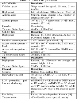
TABLE I: Simulation parameters

mMIMO-BSs Description

Cellular layout Wrap around hexagonal, 19 sites, 3 sec-tors/site

Deployment Inter-site distance:500m, height:32m [16] Antenna array Uniform linear, spacing:0.5λ, Number of

antennas per array: 64

Antenna pattern 70◦_{H x}10◦_{V beamwidths, 14}dBimax., downtilt:15◦_[16]

Precoder Zero-forcing

Tx power/Noise figure 46 dBm, 5 dBm [16] Self-BH SCs Description

Deployment Random:{4,8,16}SCs/sector, Ad-hoc: 16 SCs/sector, height:5m

Backhaul antenna pattern 5dBiantenna gain, Omni [16] Access antenna pattern –

Patch

80◦ _{H x}80◦_{V beamwidths, 5}dBimax., downtilt:90◦

Access antenna pattern – Yagi

58◦_{H x}47◦_{V beamwidths, 10}dBimax., downtilt:90◦

Tx power/Noise figure 30 dBm, 5 dB [16]

UEs Description

Deployment Random, 16 UEs/sector on average, all served, height:1.5m

Tx power/Noise figure 23 dBm, 9 dB [16]

Channel Description

Scenario Outdoor SCs, outdoor UEs

Bandwidth/Time-slot 10 MHz at 2 GHz,Qt= 50RBs,T = 1 msec. [16]

LOS probability, path loss and shadowing

mMIMO-BS to UE (based on 3GPP macro to UE models), mMIMO-BS to SC (based on 3GPP macro to relay models), SC to UE (based on 3GPP relay to UE models) as per [16]

Fast fading Rician, distance-dependent K-factor [18] Thermal noise -174 dBm/Hz power spectral density

benefit from more radio resources allocated. In fact, with more SCs, there are less UEs served per SC, and the SC can allocate more RBs per UE. However, adding more SCs increase the probability of having a larger number of interfering SCs with a LOS channel with respect to the UE. As a result, the power of the interference links grows faster than the carrier signal power due to NLOS to LOS transition of the interference links [21]. The gains provided by more radio resources and proximity are outweighed by the detrimental impact of interference, and from the curves shown in Fig. 3, we can see that the end-to-end UE rates increase marginally when doubling the number of SCs deployed.

end-to-end users rate [Mbps]

0 5 10 15 20 25 30 35 40

C

D

F

0 0.1 0.2 0.3 0.4 0.5 0.6 0.7 0.8 0.9 1

Ad-hoc,d=10 m, Patch Ant Ad-hoc,d=2.5 m, Patch Ant Ad-hoc,d_{=0 m, Patch Ant} Ad-hoc,d_{=0 m, Yagi Ant} Random, 4 SC/Sector Random, 8 SC/Sector Random, 16 SC/Sector

Fig. 3: CDF of end-to-end UE rate in: (i_{) ad-hoc deployment of} 16 SCs per sector with variable UE-to-SC distance d_{and different} antenna patterns (Patch and Yagi); (ii_{) random deployment of SCs.}

B. Impact of the resource allocation

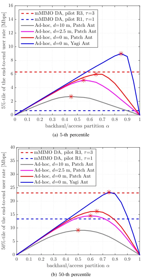
In Fig. 4, we vary α in the range 0 ≤ α≤ 1 to analyse the behaviour of UEs rate at the 5-th and 50-th percentiles of the CDF. The configurationsα= 0andα= 1entail that all the time-slots are allocated to the access and the backhaul, respectively. Therefore, the UE rate for these two values is equal to 0, since no resources are left for the other link. Fig. 4 brings the following insights:

• The s-BH links are generally the bottleneck of the two

hop connection when the SCs are densely deployed near the UEs. In such a case, in order to take advantage of the very high SINR experienced by the UEs on the access link, most of the resources must be allocated to the backhaul. For instance, withd= 0and Yagi antennas at the SCs, α∗_{, i.e., the value of αthat maximizes the}

UE rate, is about 0.85 when looking at the5-th percentile curve.

• By comparing the results between Fig. 4a and Fig. 4b, it is important to notice that the optimalαchanges from 0.85 to 0.75. This deviation suggests that picking a non-optimalαcan lead to a significant reduction of the end-to-end UE rates. In fact, assuming that the network uses α= 0.85, which is the optimal value for cell-edge UEs (5-th percentile of the CDF), the median UEs (50-th percentile of the CDF) can achieve an end-to-end rate of 19.5 Mbps, which represents a 16% reduction with respect to the maximum end-to-end rate achievable of 23.3 Mbps.

• In Figs. 4a and 4b, we show with dash lines the results

of the mMIMO DA setup, which is considered as the baseline for the network performance. The results show that a properly designed s-BH system can improve the performance of the cell-edge UEs, but this is not the case for the median-UEs. A more detailed comparison is further developed in the next section.

backhaul/access partitionα

0 0.1 0.2 0.3 0.4 0.5 0.6 0.7 0.8 0.9 1

5

%

-t

il

e

o

f

th

e

en

d

-t

o

-e

n

d

u

se

r

ra

te

[M

b

p

s]

0 2 4 6 8 10 12 14 16

mMIMO DA, pilot R3,τ=3

mMIMO DA, pilot R1,τ=1

Ad-hoc,d_{=10 m, Patch Ant} Ad-hoc,d_{=2.5 m, Patch Ant} Ad-hoc,d_{=0 m, Patch Ant} Ad-hoc,d_{=0 m, Yagi Ant}

(a)5-th percentile

backhaul/access partitionα

0 0.1 0.2 0.3 0.4 0.5 0.6 0.7 0.8 0.9 1

5

0

%

-t

il

e

o

f

th

e

en

d

-t

o

-e

n

d

u

se

r

ra

te

[M

b

p

s]

0 5 10 15 20 25 30 35 40

mMIMO DA, pilot R3,τ=3

mMIMO DA, pilot R1,τ=1

Ad-hoc,d=10 m, Patch Ant Ad-hoc,d=2.5 m, Patch Ant Ad-hoc,d=0 m, Patch Ant Ad-hoc,d_{=0 m, Yagi Ant}

(b)50-th percentile

Fig. 4: (a)5-th, and (b)50-th percentile of the UE rates as a function of the partitionα_{between backhaul and access time-slots.}

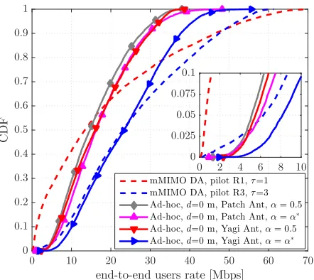
C. Comparison between DA and s-BH systems

In this section, we further compare the mMIMO s-BH and the mMIMO DA architectures to identify in which conditions the network results in a better performance in terms of UE rates. For the mMIMO DA architecture, Ki = 16 UEs are trained and served per time-slotT. From Fig. 5, we identify two different regions:

• At the bottom of the CDF, i.e. below the50-th percentile,

end-to-end users rate [Mbps]

0 10 20 30 40 50 60 70

C

D

F

0 0.1 0.2 0.3 0.4 0.5 0.6 0.7 0.8 0.9 1

0 2 4 6 8 10

0 0.025 0.05 0.075 0.1

mMIMO DA, pilot R1,τ=1

mMIMO DA, pilot R3,τ=3

Ad-hoc,d=0 m, Patch Ant,α= 0.5 Ad-hoc,d_{=0 m, Patch Ant,}α=α∗

Ad-hoc,d=0 m, Yagi Ant,α= 0.5 Ad-hoc,d=0 m, Yagi Ant,α=α∗

Fig. 5: Two types of curves are represented: (i_{) mMIMO DA with} pilot reuse schemes 1 and 3; (ii_{) ad-hoc deployment of 16 SCs per} sector forα= 0.5andα=α∗_{, at which the50-th percentile of the} UE rate is maximized (as shown in Fig. 4b).

LOS propagation condition, and 2) backhaul links benefit from the absence of pilot contamination, and the higher height of the SC compared to the UE. The latter leads to an improved path-loss and LOS conditions with respect to those modelled for the macro to UE link [16]. The gain achieved by mMIMO s-BH decreases when mMIMO DA with pilot reuse 3 is considered, mainly because of the reduced pilot contamination effect in the latter. However, we still observe some considerable gain of about 30%

withd= 0and Yagi antennas when looking at the 5-th percentile of the UE rate.

• At the top of the CDF, i.e. over the 50-th percentile, the mMIMO DA architecture exceeds the performance of s-BH mMIMO. This is because, with s-s-BH, the end-to-end rates are conditioned by both inter-cell interference and limited backhaul capacity, which combined set a limit to the maximum rate of the two hop connection.

The results of Fig. 5 confirm that the deployment of s-BH architectures can be effective for serving UEs located at the cell edge and motivate the use of mMIMO DA for serving median UEs.

V. CONCLUSION

In this paper, we analyzed the performance of the mMIMO based s-BH architecture below 6 GHz frequencies. We adopted a system-level simulation approach to investigate the UE rate performance for different SC deployments, and to analyze the effect of the variation of the backhaul/access partition. We showed that end-to-end performance greatly benefits from an ad-hoc SC deployment with one SC per UE, and studied the optimal backhaul/access partition, which maximizes the end-to-end rates, for the cell-edge UEs and for the median UEs. Additionally, we also study the effect of that antenna directivity adopted at the SCs, which leads

to important gains in a dense deployment of SCs. Finally, we compared the s-BH architecture against a mMIMO DA baseline. By properly optimizing the SC deployment and antenna directivity, s-BH outperforms DA at the cell edge in ultra-dense deployments, in particular when pilot reuse 1 is used in the latter. On the other hand, DA outperforms s-BH when looking at the median UEs.

REFERENCES

[1] A. Guptaet al., “A survey of 5G network: Architecture and emerging technologies,”IEEE Access, vol. 3, pp. 1206–1232, Jul 2015. [2] F. Ruseket al., “Scaling up MIMO: Opportunities and challenges with

very large arrays,” IEEE Signal Processing Magazine, vol. 30, no. 1, pp. 40–60, Jan 2013.

[3] D. Lopez-Perezet al., “Towards 1 Gbps/UE in cellular systems: Under-standing ultra-dense small cell deployments,”IEEE Signal Processing Mag., vol. 17, no. 4, pp. 2078–2101, 4th Quart., 2015.

[4] U. Siddiqueet al., “Wireless backhauling of 5G small cells: challenges and solution approaches,” IEEE Wireless Communications, vol. 22, no. 5, pp. 22–31, Oct 2015.

[5] N. Wanget al., “Backhauling 5G small cells: A radio resource man-agement perspective,” IEEE Wireless Communications, vol. 22, no. 5, pp. 41–49, Oct 2015.

[6] 3GPP 22.261, “Service requirements for the 5G system,” Technical Specification (TS), Sep 2017.

[7] R. Guptaet al., “Resource allocation for self-backhauled networks with half-duplex small cells,” inProc. IEEE Int. Conf. Commun. (ICC), May 2017, pp. 198–204.

[8] T. M. Nguyenet al., “Resource allocation in two-tier wireless backhaul heterogeneous networks,” IEEE Trans. Wireless Commun., vol. 15, no. 10, pp. 6690–6704, Oct 2016.

[9] P. Kelaet al., “Flexible backhauling with massive MIMO for ultra-dense networks,”IEEE Access, vol. 4, pp. 9625–9634, Dec 2016.

[10] H. H. Yanget al., “Energy-efficient design of MIMO heterogeneous networks with wireless backhaul,” IEEE Trans. Wireless Commun., vol. 15, no. 7, pp. 4914–4927, July 2016.

[11] M. Feng et al., “Joint frame design, resource allocation and user association for massive mimo heterogeneous networks with wireless backhaul,” IEEE Transactions on Wireless Communications, vol. 17, no. 3, pp. 1937–1950, March 2018.

[12] H. Tabassum et al., “Analysis of massive MIMO-enabled downlink wireless backhauling for full-duplex small cells,”IEEE Trans. Commun., vol. 64, no. 6, pp. 2354–2369, June 2016.

[13] B. Liet al., “Small cell in-band wireless backhaul in massive MIMO systems: A cooperation of next-generation techniques,” IEEE Trans. Wireless Commun., vol. 14, no. 12, pp. 7057–7069, Dec 2015. [14] W. Lv et al., “Interference coordination in full-duplex HetNet with

large-scale antenna arrays,” in2017 IEEE International Conference on Communications (ICC), May 2017, pp. 1–6.

[15] Y. G. Limet al., “Performance analysis of massive MIMO for cell-boundary users,”IEEE Trans. Wireless Commun., vol. 14, no. 12, pp. 6827–6842, Dec 2015.

[16] 3GPP 36.814, “Further advancements for E-UTRA physical layer as-pects,” Technical Report (TR), Mar 2017.

[17] I. Bor-Yalinizet al., “The new frontier in RAN heterogeneity: Multi-tier drone-cells,”IEEE Communications Magazine, vol. 54, no. 11, pp. 48–55, November 2016.

[18] 3GPP 25.996, “Spatial channel model for Multiple Input Multiple Output (MIMO) simulations (Release 14),” Technical Report (TR), Mar 2017.

[19] X. Zhu et al., “Soft pilot reuse and multicell block diagonalization precoding for massive MIMO systems,” IEEE Trans. Veh. Technol., vol. 65, no. 5, pp. 3285–3298, May 2016.

[20] L. G. Giordanoet al., “Uplink sounding reference signal coordination to combat pilot contamination in 5G massive MIMO,” in 2018 IEEE Wireless Communications and Networking Conference (WCNC), April 2018, pp. 1–6.