Exploiting Structure in Parsing to 1 Endpoint Crossing Graphs

Exploiting Structure in Parsing to 1-Endpoint-Crossing Graphs

Robin Kurtz and Marco Kuhlmann

Department of Computer and Information Science Link¨oping University, Sweden

[email protected] and [email protected]

Abstract

Deep dependency parsing can be cast as the search for maximum acyclic subgraphs in weighted digraphs. Because this search problem is intractable in the general case, we consider its restriction to the class of 1-endpoint-crossing (1ec) graphs, which has high coverage on standard data sets. Our main contribution is a characterization of 1ec graphs as a subclass of the graphs with pagenumber at most 3. Building on this we show how to extend an existing parsing al-gorithm for 1-endpoint-crossing trees to the full class. While the runtime complexity of the extended algorithm is polynomial in the length of the input sentence, it features a large constant, which poses a challenge for practical implementations.

1 Introduction

Motivated by applications in natural language un-derstanding, recent work in dependency parsing has targeted ‘deep’ graphs, a term used to refer to representations that are not necessarily tree-shaped. Such graphs support intuitive analyses of argument sharing in control constructions, quantification, and semantic modification, among others. Data sets of deep dependency graphs are often derived from the derivations of expressive grammar formalisms; for an overview, see Kuhlmann and Oepen (2016).

Deep dependency parsing has been formalized as the search for maximum acyclic subgraphs in weighted digraphs (Schluter, 2014; Kuhlmann and Jonsson, 2015). Because this problem is known to be intractable in the general case (Guruswami et al., 2011), it is interesting to identify structural restrictions on the target graphs that can yield poly-nomial-time parsing algorithms without sacrificing too much of the empirical coverage.

Schluter (2015) and Kuhlmann and Jonsson (2015) propose to address deep dependency pars-ing under the restriction that the target structures should benoncrossing, a constraint related to pro-jectivity as known from syntactic parsing. When the search space is restricted to the class of non-crossing graphs, maximum subgraph parsing is pos-sible in timeO(n3_{), wherenis the length of the}

input sentence. Unfortunately, the restriction to noncrossing graphs excludes a large proportion of the linguistic data. It seems clear that deep depen-dency parsing, much more than syntactic parsing, needs algorithms that can handle graphs with cross-ing arcs.

An interesting weaker restriction than the non-crossing condition is the restriction to graphs which are1-endpoint-crossing(Pitler et al., 2013), a con-straint originally formulated for tree-shaped graphs. The maximum 1-endpoint-crossing subtree of a weighted digraph can be found in timeO(n4_{). In}

this paper we show how to generalize this result to non-trees. This is not straightforward, as the ob-vious modification of existing algorithm for trees turns out to be incomplete for general graphs. The key to a complete algorithm, and our main techni-cal contribution, is a characterization of 1-endpoint-crossing graphs as a certain subset of the class of graphs withpagenumber at most 3(Section 3). The exact characterization refers to the restricted pat-terns in which arcs can cross each other. From this characterization we obtain anO(n5_{)algorithm for}

general graphs (Section 4). When a certain, rare type of crossing configurations is ruled out, the run-time complexity of the algorithm reduces toO(n4_),

the same as for trees.

While the runtime of both new algorithms is polynomial in the length of the input sentence, both feature large constants, which leads us to discuss challenges in extending our algorithm into a practi-cal parser for deep dependency parsing (Section 5).

Chief executives and presidents had come and gone

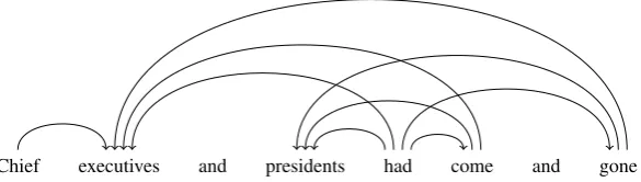
Figure 1: A sample dependency graph (Flickinger et al., 2016, CCD #20604004), drawn as an arc diagram. Note that each word is meant to represent one endpoint. (We leave some space between different arcs that share a common endpoint.) To save some space we draw arcs as semi-ellipses rather than semi-circles. The graph has pagenumber 3 and is 1ec.

2 Background

We start by giving some background on the classes of graphs that we study in this paper.

2.1 Graph Classes

A dependency graph for a natural language sen-tencexis an acyclic digraph whose vertices are in one-to-one correspondence with the words inx.1_A sample dependency graph is shown in Figure 1. To draw a dependency graph, we place its vertices on an invisible line in the plane according to their left-to-right order, and draw each arc as a semi-circle in the half-plane bounded by that line. We refer to this type of drawing as anarc diagram. Given an arc di-agram of a dependency graph, two arcs of the graph are said tocrossif their corresponding semi-circles intersect in points other than a common endpoint. A dependency graph is called noncrossing if its arc diagram does not feature crossing arcs. Noncrossing graphs have also been called ‘planar’ (Titov et al., 2009). We can generalize the non-crossing condition by allowing arcs to be drawn not only in the half-plane above the vertex line but also in that below it, or in any of some fixed num-ber k of half-planes bounded by the vertex line. This type of graph drawing is known as a book embedding(Bernhart and Kainen, 1979). (We may picture the half-planes as the pages of a book, and the vertex line as the book spine.) Thepagenumber of a graph is the smallest numberkfor which the graph has a crossing-free book embedding with khalf-planes (pages). The graph in Figure 1 has pagenumber 3. Graphs whose pagenumber is at mostkhave also been called ‘k-planar’ (G´omez-Rodr´ıguez and Nivre, 2010).

1_{We restrict our attention to unlabelled dependency graphs.}

Our main interest in this paper is in the class of 1-endpoint-crossing graphs. A dependency graph is called1-endpoint-crossing (1ec)if for each of its arcsa, all arcs that cross ashare a common endpoint (Pitler et al., 2013). The graph in Figure 1 is 1ec. The 1ec property was originally formulated for dependency trees, but the definition carries over to more general graphs without modifications.

2.2 Empirical Coverage

We assess the emprical coverage of 1ec graphs on a standard data set, the data used for the 2015 Sem-Eval Task on Broad-Coverage Dependency Parsing (Flickinger et al., 2016). This data consists of to-ken-aligned dependency graphs from four distinct linguistic traditions, dubbed DM, PAS, PSD, and CCD. For details about these target representations we refer to Oepen et al. (2016).

Table 1 gives the percentages of complete graphs (G) and individual arcs (A) that can be covered un-der the restriction to noncrossing graphs, graphs with bounded pagenumber (≤2), and 1ec graphs.2 We see that the coverage of 1ec graphs clearly sur-passes that of noncrossing graphs on all four repre-sentation types. Noncrossing graphs in fact seem to be a rather poor match for the data, especially on CCD, where it rules out more than half of the target graphs. With respect to pagenumber, even the low bound at≤2 achieves very highest coverage, the highest among the three classes considered. The class 1ec is on average 2.11 percentage points be-hind in terms of coverage on complete graphs and 0.14 points on individual arcs.

class DM PAS PSD CCD nc G 69.29 59.85 65.04 49.53 A 97.63 97.24 96.01 95.83 pn≤2 G 99.46 99.48 97.64 98.33 A 99.97 99.97 99.76 99.89 1ec G 97.30 97.18 95.85 96.16 A 99.83 99.85 99.60 99.75

Table 1: Coverage in terms of complete graphs (G) and individual arcs (A) for noncrossing graphs, graphs with pagenumber at most 2, and 1ec graphs.

2.3 Parsing Complexity

While high coverage is desirable, it often goes hand in hand with high parsing complexity. As already mentioned in the introduction, the maximum non-crossing subgraph can be found in time O(n3_),

wherenis the length of the input sentence. The corresponding problem for the class of graphs with pagenumber at most 2 is NP-hard (Kuhlmann and Jonsson, 2015), which means that the high cov-erage of this class incurs a considerable price to pay. The relatively high coverage of 1ec graphs ob-served in Table 1 suggests that this class of graphs might strike a good balance between coverage and complexity.

3 The Structure of 1ec Graphs

In this section we derive the structural character-ization of 1ec graphs that we will exploit in our parsing algorithm. Our point of departure is the result of Pitler et al. (2013, Theorem 1) that 1ec trees have pagenumber at most 2. This result does not carry over to general graphs; in fact we have already seen an empirical example of a 1ec graph with pagenumber 3 in Figure 1.

Lemma 1 There are 1ec graphs with

pagenum-ber 3. 2

Our first goal is to prove that pagenumber 3 is also themaximal pagenumber of 1ec graphs. To show this we will characterize 1ec graphs in terms of theircrossing graphs.

3.1 Pagenumber of 1ec Graphs

Thecrossing graphof a dependency graph has a vertex corresponding to each arc, and an edge be-tween two vertices if and only if the corresponding arcs cross. The crossing graphs of noncrossing dependency graphs consist of isolated vertices.

Crossing graphs are interesting because the pa-genumber of a dependency graph equals the chro-matic number of its crossing graph, the smallest number of colours needed to colour the vertices of the crossing graph in such a way that no two neighbouring vertices share the same colour. From a k-colouring of its crossing graph we obtain a crossing-freek-book embedding of the dependency graph by placing two arcs on the same page if and only if their corresponding vertices are coloured with the same colour. This correspondence has previously been studied by G´omez-Rodr´ıguez and Nivre (2010) and Kuhlmann and Jonsson (2015), among others. The following lemma is due to Pitler et al. (2013, Lemma 2).

Lemma 2 The crossing graphs of 1ec graphs do not contain triangles (cycles of length 3). 2

PROOF Suppose for the sake of contradiction that there exists a cycleabca. The arcsaandcmust share an endpoint, as they both crossb. Because of this, they cannot cross, and therefore cannot be

adjacent in the cycle.

We use this lemma in the proof of the following:

Lemma 3 The pagenumber of 1ec graphs is at

most 3. 2

PROOF We show that the crossing graph of a 1ec graph is 3-colourable. To colour the crossing graph, we separately colour each of its components (also crossing graphs). We distinguish two cases:

1. The component does not contain a cycle, or contains cycles of length at most 4. By Lemma 2, the component does not contain a triangle, and therefore no odd cycle at all. We can therefore 2-colour the component by traversing the component using depth-first search and assigning to each vertex the op-posite colour of its parent in the search tree.

2. The length of the shortest cycle in the compo-nent is at least 5. In the graph theory literature, our crossing graphs are better known ascircle graphs, and the length of the shortest cycle in a graph is known as itsgirth. It has been shown that every circle graph with girth at least 5 is 3-colourable (Ageev, 1999).

1 2 3 4 5

•

1

• 2

•

3

•

4

•

5

•

(1,3)

•(2,4)

•

(3,5)

•

(4,1)

•

(2,5)

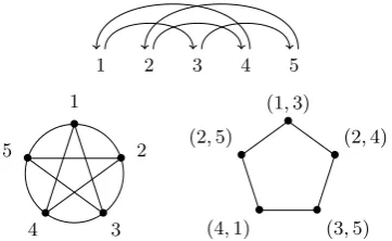
Figure 2: Counter-clockwise from top: dependency graph, chord diagram, crossing graph.

3.2 Isolation Property for Cog Belts

1ec graphs with pagenumber 3 (or subgraphs thereof) have a characteristic structure reminiscent of the teeth of a cogwheel; a minimal example is shown at the top of Figure 2. The proof of Lemma 3 also reveals that these graphs correspond to cycles of length 5 or more in the crossing graph. Because of this we will refer to these graphs ascog belts. Our aim for the remainder of this section is to show (in Lemma 6) that these structures are ‘isolated’, in the sense that no arcs other than the arcs in the cog belt can cross the cog belt. This property will be the key to the parsing algorithm in Section 4. To show it we study the relation between crossing graphs andchord diagrams.

The chord diagram of a dependency graph is obtained by placing the vertices of the graph on the boundary of a circle such that their clockwise order extends the left-to-right order in the original graph, and drawing each arc of the graph as a chord of the circle. An example is given in Figure 2. Note that the chord diagram representation does not contain information about the direction of the arcs of the de-pendency graph, and cannot be used to recover the exact linear positions of the vertices. Importantly though, we can still read off the crossing graph of a dependency graph from its chord diagram.

To prove the maximality property, we will reason about the chord diagram corresponding to a cross-ing graph. In general, this diagram is not uniquely determined. However, when we restrict ourselves to ‘strict’ chord diagrams in which there are ex-actly twice as many endpoints as there are chords, then there are certain crossing graphs that have a uniquesuch chord diagram (up to symmetry).3 _In particular, this holds for cycles of length at least 5.

3_{These are exactly the graphs that areprimewith respect} to split decompositions; see Gabor et al. (1989).

We start by proving a lemma about another type of graphs with unique strict chord diagrams. A dominois a graph of the form .

Lemma 4 The crossing graphs of 1ec graphs do

not contain dominoes. 2

PROOF For the sake of contradiction, suppose that the crossing graph of a 1ec graph G contains a domino. The arcs that correspond to the vertices on this domino induce a subgraph ofG. We rea-son about how the chord diagrams for this induced subgraph could look like. A domino has a unique ‘strict’ chord diagram (Gabor et al., 1989); this

di-agram looks as shown in the left half of Figure 3. However, this chord diagram cannot be the actual chord diagram of a 1ec dependency graph. For example, the chordb is crossed by chordsaand d, but these chords do not share a common end-point. We can try to ‘repair’ the chord diagram (without changing the underlying crossing graph) by merging some of the endpoints; in particular, we can merge the two endpoints a2 and d1 into

one endpoint that we may refer to asad, which re-moves one violation of the 1ec property at chordb. Eliminating as many violations as possible, we ob-tain the modified chord diagram in the right half of Figure 3. However, even in this diagram there are still some violations left: Apart fromaandd, the chord b is also crossed by e, and this chord cannot be made to share an endpoint withaandd. We therefore conclude that the crossing graph ofG does not contain a domino. For our next lemma we need some terminology from geometry. Apolygramis a non-convex regu-lar polygon, drawn by connecting a given number of points placed at equal distance on the bound-ary of a circle. Polygrams can be denoted by its Schl¨afli symbol{p/q}, wherepgives the number of corners, and q states that each corner should be connected to its neighboursq steps away. For example,{5/2}denotes the pentagram in Figure 2.

•

a1

•b1 •c1

•_a2 •

d1

•

c2

•

e1

•

b2

•

f1

•

e2

•

d2 •

f2

a b

c e

f d

•a1 •bc

•_ad •

c2

•

e1

•

bf

•

ed

•

f1

a b

c e

f d

• 1 •2 • 3 • ₄ • 5 • 6 • 7 • 8 • 9 _• • • 1 •2 • 3 •₄ • 5 • 6 • 7 • 8 • 9 • • • 1 •2 • 3 • ₄ • 5 • 6 • 7 • 8 • 9 • •

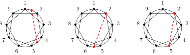
Figure 4: Proof of Lemma 6, illustrated using a cycle of lengthm= 9. The additional chord (red-dashed) violates the 1ec property: In the graph on theleft, it creates additional endpoints for the chords13,29,35, and46; in the graph in themiddle, it creates additional endpoints for the chords46and57; in the graph on theright, the new chord is crossed by13and46, which do not share an endpoint.

Lemma 5 The chord diagram of the subgraph in-duced by a cycle of lengthm ≥ 5 in a crossing graph of a 1ec graph is unique (up to symmetry) and forms a polygram{m/2}. 2

PROOF Similar to the proof of Lemma 4, we rea-son about how the chord diagrams for the subgraph induced by a cycle of lengthm ≥5in a crossing graph of a 1ec graph could look like. We illus-trate our argument using concrete cycles,abcdea (m = 5) andabcdefa(m = 6). The strict chord diagrams for these examples look as follows.

•

a1

•c1 •b1

•d1

•_c 2 • e1 • d2 • a2 • e2 • b2

a b c

d e

•

a1

•c1 •b1

•d1

•_c2 • e1 • d2 • f1 • e2 • a2 • f2 • b2

a b c

d e f

Again, these diagrams cannot be chord diagrams of 1ec dependency graphs; for example, the chord bis crossed by chordaandc, which do not have a common endpoint. The only way to repair the chord diagrams without changing the underlying crossing graph is to merge the two endpointsa1and

c1into a common endpoint which we shall refer to

asac, and likewise for all the other chords. This yields the following (non-strict) chord diagrams:

• ac •bd • ce • ad • be _b c d e a • ac •bd •_ce • df • ea • fb _b c d e f a

The left diagram is the pentagram{5/2}, the right diagram is the hexagram{6/2}(6 corners, each of which is connected to the neighbour 2 steps away).

From these examples it is not hard to generalize to arbitrary values ofm: Ifmis odd, then the chord diagram for the cycle forms a regular star polygon. Ifmis even, then the chord diagram forms a regular polygon compound consisting of two copies of a regular, convex(m/2)-gon. Pitler et al. (2013, Lemma 3) show that any odd cycle of lengthm≥5in a crossing graph of a 1ec graph uses at mostmvertices in the original graph. From Lemma 5 we get the stronger result thatany cycle of lengthm≥5usesexactlymvertices.

We are now ready to prove the isolation property:

Lemma 6 Any cycle of lengthm≥5in a crossing graph of a 1ec graph forms a connected component

of that graph. 2

4 Parsing Algorithm

In the previous section we have characterized 1ec graphs in terms of their crossing graphs. In this sec-tion we will exploit this characterizasec-tion to show how to obtain a parsing algorithm for 1ec graphs. We follow Kuhlmann and Jonsson (2015) in cast-ing dependency parscast-ing as a maximum subgraph problem: Given an arc-weighted digraphG, our aim is to find a subset of arcs with maximum total weight such that the induced subgraph is 1ec. The weights ofGshould be learned from data.

4.1 Relaxed Deduction System for 1ec Trees

To obtain a parsing algorithm for 1ec graphs, an obvious idea is to take the corresponding algorithm for trees (Pitler et al., 2013) and ‘relax’ it by delet-ing all book-keepdelet-ing that is used to enforce the tree constraint. We present the resulting algorithm as aweighted deduction system(Shieber et al., 1995; Nederhof, 2003). Such a system uses inference rules to derive information about sets of graphs; this information is represented by weighted formu-las calleditems. Parsing amounts to finding the derivation of a goal itemwith maximum weight, starting from a set ofinitial items.

We assume that we are given an arc-weighted digraphG= (V, A)with verticesV ={1, . . . , n}. Items represent subgraphs ofGcorresponding to ei-therisolated intervals[i, j], where there are no arcs between vertices in the open interval(i, j)and ver-tices outside of[i, j], orisolated crossing regions [i, j]∪ {x}, where there are i) no arcs between ver-tices in(i, j)and vertices outside of[i, j]∪{x}, and ii) no arcs between the external vertexxand ver-tices in(i, j)that are crossed by arcs with both end-points in(i, j). Isolated intervals are represented by items of the formInt[i, j], and isolated crossing regions are represented by four different types of items that put a constraint on whether arcs fromx into(i, j) may be crossed by arcs inside of[i, j] with endpoints at the left border (L[i, j, x]), the right border (R[i, j, x]), both borders (LR[i, j, x]), or none of the two borders (N[i, j, x]). The initial items of the system correspond to one-vertex sub-graphs and take the formInt[i, i]. The goal item isInt[1, n], representing the complete graph that spans all vertices. Finally, the inference rules are shown in Figure 6. The weight of the item on the left-hand side of each rule is computed as the sum of weights of the items on the right-hand side and, if specified, the weight of a new arc.

1 2 3 4 5 6

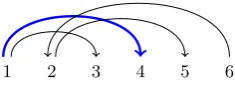
Figure 5: Non-completeness for general 1ec graphs. Splitting the itemLR[1,5,6]atk = 3using rule (11) makes it impossible to retain the arc2←4.

4.2 Non-Completeness for General Graphs

A deduction system is correct with respect to a class of graphsGif each of its derivations denotes (under an intended interpretation) a graph fromG (soundness), and every graph fromG has some derivation (completeness). While the algorithm of Pitler et al. (2013) is correct for the class of 1ec trees, it turns out that its relaxed version is notcorrect for the full class of 1ec graphs. More specifically, there are some 1ec graphs that do not have derivations in the relaxed system.

To illustrate the problem, we consider the cog belt in Figure 5 and reason backwards, reading inference rules as rules fordecomposinga subgraph into smaller ones. The only way to decompose the example graph from anInt item is to instantiate rule (6) withk= 5. This removes the dashed arc 5→1, leaving the rest of the graph inside anLR

item. Now to decompose theLRitem we need to find a ‘split vertex’k∈(1,5)for rule (11), creating itemsL[1, k,6]andR[k,5,6]. However, splitting the graph in this way makes it impossible to retain arcs that cover k – and inside the interval (1,5) everyvertex is covered by some arc. This property prevents the decomposition of not only the graph in Figure 5, but more generally every cog belt.

4.3 Correctness for Graphs without Cog Belts

While the relaxed deduction system is not correct for general 1ec graphs, we can prove that it is cor-rect for the class of all 1ec graphs that do not con-tain cog belts. The proof is straightforward but te-dious, so here we content ourselves with sketching the structure and giving the most central intuitions.

(1) Int[i, j]←Int[i+ 1, j]

(2) Int[i, j]←s[i, j] +Int[i, j]

(3) Int[i, j]←s[i, k] +Int[i, k] +Int[k, j]

(4) Int[i, j]←s[i, k] +R[i, k, l] +Int[k, l] +L[l, j, k]

(5) Int[i, j]←s[i, k] +LR[i, k, l] +Int[k, l] +Int[l, j]

(6) Int[i, j]←s[i, k] +LR[i, k, j] +Int[k, j]

(7) Int[i, j]←s[i, k] +Int[i, l] +L[l, k, i] +N[k, j, l]

(8) Int[i, j]←s[i, k] +R[i, l, k] +Int[l, k] +L[k, j, l]

(9) LR[i, j, x]←R[i, j, x]

(10) LR[i, j, x]←L[i, j, x]

(11) LR[i, j, x]←L[i, k, x] +R[k, j, x]

(12) N[i, j, x]←s[x, k] +N[i, k, x] +Int[k, j]

(13) N[i, j, x]←Int[i, j]

(14) N[i, j, x]←s[i, x] +N[i, j, x]

(15) N[i, j, x]←s[j, x] +N[i, j, x]

(16) L[i, j, x]←Int[i, j]

(17) L[i, j, x]←s[x, k] +L[i, k, x] +Int[k, j]

(18) L[i, j, x]←s[i, k] +L[i, k, x] +Int[k, j]

(19) L[i, j, x]←s[x, k] +Int[i, k] +L[k, j, i]

(20) L[i, j, x]←s[i, x] +L[i, j, x]

(21) L[i, j, x]←s[j, x] +L[i, j, x]

(22) L[i, j, x]←s[i, j] +L[i, j, x]

(23) R[i, j, x]←Int[i, j]

(24) R[i, j, x]←s[x, k] +Int[i, k] +R[k, j, x]

(25) R[i, j, x]←s[j, k] +Int[i, k] +R[k, j, x]

(26) R[i, j, x]←s[x, k] +R[i, k, j] +Int[k, j]

(27) R[i, j, x]←s[i, x] +R[i, j, x]

(28) R[i, j, x]←s[j, x] +R[i, j, x]

(29) R[i, j, x]←s[i, j] +R[i, j, x]

Figure 6: The rules of the ‘relaxed’ deduction system, following the basic rules of Pitler (2013). The scores for arcss[i, j]do not specify the arc’s direction (we simply choose the arc with the higher weight). The indices may not overlap, giving rise to rule (6), the special case of rule (5) forl=j.

inherited from the tree-based system. Showing that the rule applications cannot result in cog belts is slightly more complicated. However, we can con-vince ourselves that the constraints implied by the item types and the constraints on the accessibil-ity of vertices implied in the rules are sufficient to exclude the forbidden structures. In particular, a derivation cannot ‘remember’ the vertex that would be needed to close off a cog belt (see Figure 7).

Completeness To show that every 1ec graph without cog belts can be derived by the system, we use induction on the size of the graph, where size is measured as the total number of vertices

1 2 3 4 5 6

Figure 7: When attempting to derive this cog belt right-to-left we could instantiate rule (8) as

Int[1,6]←s[1,3]+R[1,2,3]+Int[2,3]+L[3,6,2] which would add the blue arc. However, the right endpoint of the red arc (5) is no longer ‘visible’.

and arcs. Graphs with size 1 (one vertex) are repre-sented by the initial items. For the inductive case we need to check that every graph which satisfies the structural property is decomposable by some rule. We can use the same strategy as Pitler (2013), who classifies graphs into a number of templates and for each of those templates shows which rule can be applied to it. In particular we need to show that the subgraphs gained in each decomposition adhere to the intended interpretations, and that all arcs can be added. The important observation is that, if the graph does not contain a cog belt, then the information represented in each item is suffi-cient to build all arcs (see Figure 8).

1 2 3 4 5 6

Figure 8: This dependency graph has a crossing graph with a cycle of length 4 and is therefore ‘almost as hard’ as a cog belt. It can be derived in the relaxed deduction system using rule (7):

(30) C[i, j, x, y]←s[x, y] +s[i, j] +Int[i, y] +Int[y, j]

(31) C[i, j, x, y]←s[x, k] +Int[i, k] +C[k, j, i, y]

(32) Int[i, j]←s[i, k] +s[i, y] +s[l, j] +Int[i, l] +Int[l, k] +C[k, j, l, y]

Figure 9: Additional rules for cog belts.

4.4 Extension to the Full Class

We have just seen that the subgraphs which the relaxed deduction system fails to parse are exactly cog belts. We now show how to extend the sys-tem into a complete parser for the full class of 1ec graphs. The key idea is that because cog belts are isolated from the remainder of the graph in terms of crossing arcs as per Lemma 6, we can simply add new items and rules that build a cog belt on top of a set of isolated intervals.

The new items take the formC[i, j, x, y]and rep-resent partial cog belts on an interval[i, j]with two additional vertices: one external vertexx(which always lies to the left ofi) and one new internal vertexy, whose purpose is to ‘remember’ the ver-tex that will be needed to close the cog belt (cf. Figure 7). The new inference rules are given in Figure 9 and are set up to derive a cog belt right-to-left. Rule (30) starts the derivation, combining two isolated intervals and adding two arcs. Rule (31) ex-tends the cog belt by one isolated interval, adding a new arc. Finally, rule (32) closes the cog belt by adding two final intervals and three new arcs. With this simple extension, the deduction system becomes sound and complete with respect to the full class of 1ec graphs.

Example derivation. To illustrate the workings of the new rules, we provide a derivation of a cog belt with length 6, which in Figure 5 we showed to be non-derivable in the relaxed system. We as-sume that we have already derived isolated interval itemsInt[i, i+ 1]for all verticesi < n. We then instantiate rule (30) as

C[4,6,3,5]←s[3,5] +s[4,6]

+Int[4,5] +Int[5,6] and after that rule (31) as

C[3,6,2,5]←s[2,4] +Int[3,4] +C[4,6,3,5] To complete the derivation of the cog belt as a closed interval item we instantiate rule (32) as

Int[1,6]←s[1,3] +s[1,5] +s[2,6]

+Int[1,2] +Int[2,3] +C[3,6,2,5]

The asymptotic runtime complexity of the ex-tended algorithm is inO(n5_{), one order of}

magni-tude higher than that of the tree-based algorithm. This is due to rules (31) and (32), each of which refers to five independent positions in the sentence.

5 Discussion

In this section we discuss our results and relate them to other published work.

5.1 Graph-Theoretical Results

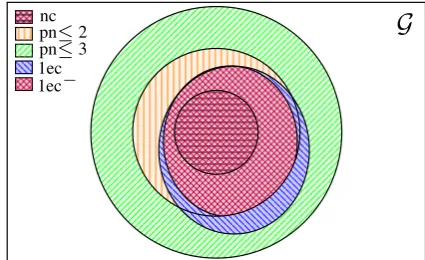
The main technical contribution of this paper is a characterization of 1ec graphs as a subclass of graphs with pagenumber at most 3 via certain prop-erties of their crossing graphs – in particular the absence of dominoes and the isolation of cycles of length at least five, which induce the substructures that we called cog belts (Section 3). The relations between the various graph classes discussed in this paper are visualized in Figure 10.

1ec graphs have previously been discussed pri-marily in the context of dependency parsing. The characterization in this paper was established us-ing results from graph theory, in particular from the study of circle graphs (Ageev, 1999). Future work of this kind may help to identify new classes of interesting dependency graphs or new parsing algorithms.

G

nc pn≤2 pn≤3 1ec 1ec−

Two classes of graphs that appear to be very relevant for the study of 1ec graphs are fan-pla-nar graphs(Kaufmann and Ueckerdt, 2014) and outer-fan-planar graphs(Bekos et al., 2014). Their defining property is essentially identical to the 1ec constraint; however, their vertices are not linearly ordered as in dependency graphs,

5.2 Parsing Algorithm

A second contribution of this paper is the exten-sion of the parsing algorithm for 1ec trees (Pitler et al., 2013) to a quintic-time algorithm for the full class of 1ec graphs, and a quartic-time algorithm for the restricted class of 1ec graphs without cog belts. Closely related algorithms were recently pro-posed by Cao et al. (2017) and Kummerfeld and Klein (2017). The former use an approach simi-lar to ours in Section 4.4 to parse what they call ‘coupled staggered patterns’ (our cog belts), albeit restricted to pagenumber 2; they report state-of-the-art results on the SemEval data. Kummerfeld and Klein (2017) apply 1ec graphs in the context of parsing to phrase structure representations with traces; their algorithm cannot parse what they call ‘locked chains’ (our cog belts), but has the benefit

of enforcing acyclicity and uniqueness.

The proposed quintic-time algorithm may not be the most attractive one for practical parsing. We looked at the SemEval data from Section 2 and found that cog belts occur rarely, less than once per 2,000 sentences, and for only two of the representa-tion types (PSD and CCD). A similar observarepresenta-tion was made by Kummerfeld and Klein (2017) for the graphs they obtained from their treebank data.

In presenting our algorithms, our main focus was on theoretical properties (soundness and complete-ness). To support the implementation of a practical parser, the extended deduction system needs to be refined in several ways. For one thing, the system features a high degree of derivational ambiguity, which in particular can lead to the same arc being scored several times in a derivation. To avoid this, we would need to extend the items with informa-tion on whether an arc has already been set, very similar to the booleans used to control treeness in the original algorithm. For example, a modified version of rule (5) could look like this:

Int[i, j;F]←s[i, k] +LR[i, k, l;F, bi,l, bk,l]

+Int[k, l;F] +Int[l, j;bl,j]

TheLRitem has three booleans, corresponding to

the three arcs that could be present among the three sets of endpoints{i, k},{i, l}, and{k, l}. The first boolean has to beF (false), as the arc between iand k is scored in the rule; the other two arcs may or may not be already present, so the values of the second and third boolean are free to choose. However, when the arc betweenkandlwas set in the derivation of theLRitem, it should not have been already set in the derivation of theInt[k, l] item, which is why we need to set the boolean in this item toF.

The modified version of rule (5) is actually a rule templatewhich in an actual parser implemen-tation needs to be instantiated in all legal ways. This introduces a non-negligible constant factor into the runtime: assuming a minimal number of three boolean variables per rule and a fourth bi-nary choice for the direction of the arc (which we have left underspecified), we would already get 32·24 _{= 512 actual rules. This ignores the}

ad-ditional bookkeeping that needs to be added in order to prevent cycles or enforce uniqueness of derivations, each of which would at least double the number of rules, and the increased complexity coming from labelled parsing.

The most promising parsing results so far on the SDP data have been achieved with a simple, quadratic-time parsing algorithm with very few constraints on the search space but a strong learn-ing component (Martins and Almeida, 2014; Peng et al., 2017). A structurally restricted parsing algo-rithm such as the one described in this paper, even if its coverage is high, has the drawback that it is harder to combine with an expressive learning ap-proach such as the recurrent neural networks used by Kiperwasser and Goldberg (2016).

6 Conclusion

Acknowledgements

We thank the anonymous reviewers for their helpful comments. This work was supported by a Google Faculty Research Award to Marco Kuhlmann.

References

Alexander A. Ageev. 1999. Every circle graph of girth at least 5 is 3-colourable. Discrete Mathematics 195(1–3):229–233.

Michael A. Bekos, Sabine Cornelsen, Luca Grilli, Seok-Hee Hong, and Michael Kaufmann. 2014. On the recognition of fan-planar and maximal outer-fan-planar graphs. InGraph Drawing. Springer, volume 8871 of Lecture Notes in Computer Science, pages 198–209.

Frank Bernhart and Paul C. Kainen. 1979. The book thickness of a graph.Journal of Combinatorial The-ory, Series B27(3):320–331.

Junjie Cao, Sheng Huang, Weiwei Sun, and Xiao-jun Wan. 2017. Parsing to 1-endpoint-crossing, pagenumber-2 graphs. InProceedings of the 55th Annual Meeting of the Association for Computa-tional Linguistics (ACL). Vancouver, Canada, pages 2110–2120.

Dan Flickinger, Jan Hajiˇc, Angelina Ivanova, Marco Kuhlmann, Yusuke Miyao, Stephan Oepen, and Daniel Zeman. 2016. SDP 2014 & 2015: Broad cov-erage semantic dependency parsing LDC2016T10. Web Download.

Csaba P. Gabor, Kenneth J. Supowit, and Wen-Lian Hsu. 1989. Recognizing circle graphs in polynomial time. Journal of the Association for Computing Ma-chinery36(3):435–473.

Carlos G´omez-Rodr´ıguez and Joakim Nivre. 2010. A transition-based parser for 2-planar dependency structures. InProceedings of the 48th Annual Meet-ing of the Association for Computational LMeet-inguistics (ACL). Uppsala, Sweden, pages 1492–1501. Venkatesan Guruswami, Johan H˚astad, Rajsekar

Manokaran, Prasad Raghavendra, and Moses Charikar. 2011. Beating the random ordering is hard: Every ordering CSP is approximation resistant. SIAM Journal on Computing40(3):878–914. Michael Kaufmann and Torsten Ueckerdt. 2014. The

density of fan-planar graphs.CoRRabs/1403.6184. Eliyahu Kiperwasser and Yoav Goldberg. 2016.

Sim-ple and accurate dependency parsing using bidirec-tional LSTM feature representations. Transactions of the Association for Computational Linguistics 4:313–327.

Marco Kuhlmann and Peter Jonsson. 2015. Parsing to noncrossing dependency graphs. Transactions of the Association for Computational Linguistics 3:559– 570.

Marco Kuhlmann and Stephan Oepen. 2016. Towards a catalogue of linguistic graph banks. Computa-tional Linguistics42(4):819–827.

Jonathan K. Kummerfeld and Dan Klein. 2017. Pars-ing with traces: AnO(n4_{)algorithm and a structural} representation. Transactions of the Association for Computational Linguistics5.

Andr´e F. T. Martins and Mariana S. C. Almeida. 2014. Priberam: A turbo semantic parser with second or-der features. InProceedings of the 8th International Workshop on Semantic Evaluation (SemEval 2014). Dublin, Republic of Ireland, pages 471–476. Mark-Jan Nederhof. 2003. Weighted deductive parsing

and Knuth’s algorithm. Computational Linguistics 29(1):135–143.

Stephan Oepen, Marco Kuhlmann, Yusuke Miyao, Daniel Zeman, Silvie Cinkov´a, Dan Flickinger, Jan Hajiˇc, Angelina Ivanova, and Zdeˇnka Ureˇsov´a. 2016. Towards comparability of linguistic graph banks for semantic parsing. In Proceedings of the 10th In-ternational Conference on Language Resources and Evaluation (LREC). Portoroˇz, Slovenia, pages 3991– 3995.

Hao Peng, Sam Thomson, and Noah A. Smith. 2017. Deep multitask learning for semantic dependency parsing. In Proceedings of the 55th Annual Meet-ing of the Association for Computational LMeet-inguistics (ACL). Vancouver, Canada, pages 2037–2048. Emily Pitler. 2013. Models for improved tractability

and accuracy in dependency parsing. Ph.D. thesis, University of Pennsylvania.

Emily Pitler, Sampath Kannan, and Mitchell Marcus. 2013. Finding optimal 1-endpoint-crossing trees. Transactions of the Association for Computational Linguistics1:13–24.

Natalie Schluter. 2014. On maximum spanning DAG algorithms for semantic DAG parsing. In Proceed-ings of the ACL 2014 Workshop on Semantic Parsing. Baltimore, USA, pages 61–65.

Natalie Schluter. 2015. The complexity of finding the maximum spanning DAG and other restrictions for DAG parsing of natural language. InProceedings of the Fourth Joint Conference on Lexical and Com-putational Semantics. Denver, CO, USA, pages 259– 268.

Stuart M. Shieber, Yves Schabes, and Fernando Pereira. 1995. Principles and implementation of deductive parsing. Journal of Logic Programming24(1–2):3– 36.