Learning to Compose Spatial Relations with Grounded Neural Language Models

Learning to Compose Spatial Relations with Grounded Neural

Language Models

Mehdi Ghanimifard CLASP

University of Gothenburg, Sweden [email protected]

Simon Dobnik CLASP

University of Gothenburg, Sweden [email protected]

Abstract

Language is compositional: we can generate and interpret novel sentences by having a notion of meaning of their individual parts. Spatial descriptions are grounded in perceptional representations but their meaning is also defined by what neighbouring words they co-occur with. In this paper we examine how language models conditioned on perceptual features can capture the semantics of com-posed phrases as well as of individual words. We generate a synthetic dataset of spatial descriptions referring to perceptual scenes and examine how grounded language models built with deep neural networks can account for compositionality of descriptions – by evaluating how the learned language models can deal with novel grounded composed descriptions and novel grounded decomposed de-scriptions, constituents previously not seen in isolation.

1

Introduction

Representing and reasoning with linguistic meaning is a central task in computational linguistics. Here

two kinds of meaning representations are used: (i)probabilistic language modelsand (ii)meaning

rep-resentations grounded in other, typically perceptual information. Recently, there have been several ap-proaches in deep learning that deal with both, either independently or together.

The main goal ofprobabilistic language modelsis to estimate a probability distribution of sequences

of words based on observable samples from language production, typically by estimating conditional probabilities of words with a categorical distribution. This gives language models means for representing words as sequences with a measure of likelihood for each sequence. Neural language models perform this objective by parametrising a probability density function with parametric representations of words and functions which compose words into phrases (Bengio et al., 2003; Mnih and Hinton, 2007; Mikolov et al., 2010). The gradient based learning in neural networks turns the modelling problem into an optimisation problem, minimising the error or distance between a model prediction and an observable data over a list of parameters:

1. parameters representing words with feature vectors known asword embeddings;

2. parameters of functions composing word features into a structure;

3. parameters of projections from final composed representations to categorical probabilities which in sequential models are the next word predictions.

There have been many attempts to show that the learned word embeddings in vector spaces are good representations of meaning. Basing the argument on the distributional hypothesis, if a probabilistic model of words is conditioned on their context words (i.e. skip-grams or bag-of-words), the word embeddings must encode semantic information by having learned distances in vector spaces which correspond to semantic similarity scores obtained through relatedness tests performed by native speakers. These

rep-resentations were extended to word compositions by considering different compositional functions as

of composition in a language model is broader than this: it involves (1) distributional models of words estimated from word sequences as well as (2) their grounding into representations of physical space. This extends the Montague’s notion of compositionality. Lexical representations and their compositions are not dependent on meaning postulates and lexicalised constraints but rather perceptual evidence which is (probabilistically) associated with them.

Harnad (1990); Roy (2005) define language grounding as a process of relating words with an agent’s perception. The ambiguity and vagueness of grounded meanings as well as of syntactic structures suggest that the connection between language and perception is gradient and therefore probabilistic. The main approaches to probabilistic models of grounded language are probabilistic learning of grounded language and grammar (Roy and Mukherjee, 2005; Matuszek et al., 2012), classifiers (Dobnik, 2009), and feature representations in perceptual space such as colour (McMahan and Stone, 2015). Our proposal is in line with all three approaches.

Agrounded language modelis a language model conditioned by perceptual representations that it refers to. Ideally, the model should capture how each constituent in the composed phrase relates to some perceptual representations. For example, in an image captioning task, a grounded language model

estimates a conditional probability of a word sequencew1:T given some image featurecthat the words

refers to. A general way to model word sequences is to use the chain rule as follows. The model can generate phrases and sentences step-by-step by predicting the next word in a sequence:

Pr(w1:T|c)= T Y

t=1

Pr(wt|w1:t,c) (1)

The parametrisation of vision and language is often done by combining word-embeddings with mul-timodal embeddings (Kiros et al., 2014; Socher et al., 2014). In the state of the art models for image captioning with encoder-decoder architecture, the encoder module is trained under the assumption that grounded words only denote features in subareas of an image, e.g bounding boxes (Karpathy and Fei-Fei, 2015) and pixel-wise mapping with attention models (Xu et al., 2015; Lu et al., 2016). Another example of a visually grounded language model is a model that is used to demonstrate the compositionality of colour descriptions in (Monroe et al., 2016) where linguistic descriptions are associated with areas of the colour space. Similar to (McMahan and Stone, 2015), each observed instance is a colour term paired with a colour code but instead of considering each description as a lexical entry, phrases are captured by a grounded language model as in Equation 1. The qualitative human evaluation of how newly com-posed colour words by this model refer to the colour space suggest that language models can capture compositionality through gradient learning used with neural networks.

In this paper, we follow up and extend the work of (Monroe et al., 2016). We focus on recurrent neu-ral language models of sequences of words conditioned by encoded locations that these words refer to in visual scenes. Hence, we are interested in grounded semantic composition that is not only captured by probabilistic models of words given their context words, but also by models of their relatedness to

percep-tual representations. An important and novel question we investigate iswhat these models are learning:

to what degree the representations of meaning (both collocational from vector spaces and grounded in

perception) are interpretable and thereforecompositionalin the sense of (Montague, 1974). We focus on

one domain of grounded meaning: spatial descriptions of various length and their grounding in spatial

templates of Logan and Sadler (1996). In particular we try to answer the following questions: (1) To

what extent are the language models that have been learned grounded in spatial representations? (2)Is

it possible to generate new, previously unseen grounded composed spatial descriptions from observing their words only in other grounded composed phrases?

This paper is organised as follows. In Section 2 we describe the creation of an artificial dataset of composed spatial templates and the associated descriptions based on the experimental work of (Lo-gan and Sadler, 1996). In Section 3 we describe our neural network model which we use for training our grounded language model. Section 4 describes an evaluation of the learned representations com-pared to the original representations the system was learning from. Finally, Section 5 points to

spatial-composition.

2

The dataset

In order to train a grounded language model we require samples of language use paired with locations they are referring to. Considering the rationality of speakers and their observers (Grice, 1975), the frequency of each co-occurring utterance–location corresponds to the appropriateness of such utterance as a description of that location. One complication of judging the appropriateness of spatial terms this way is that they are not only depended on the location they describe but also on other properties of the situation such as the agreed frame of reference, object shape, and the function of the landmark and the target objects involved, etc. (Herskovits, 1986; Dobnik and Cooper, 2017). However, these properties will not be considered in the present study.

Logan and Sadler (1996) performed several psychological experiments related to the geometric ap-prehension of spatial relations. For example, they collected acceptability ratings (1–9) for a set of spatial relations per different locations of the target object in a 7×7 grid relative to the landmark object in the

centre (3,3). The acceptability scores were collected from 32 informants through random presentation

and then averaged per location. The matrix of average acceptability scores per description is called a spatial template and represents the appropriateness of each location in the process of interpreting that spatial relation (Logan and Sadler, 1996). They collect spatial templates for the following spatial rela-tions: right of,left of,below, under,over, above, near to, next to, far from, andaway fromwhich we also apply in our work. Furthermore, in order to be able to explore the limits of the language models for learning compositions, we extend this vocabulary with a few additional words. We describe how we used them to synthesise the composed spatial templates for our training data in the following section.

2.1 Spatial templates as probabilities

As stated earlier, the spatial templates of Logan and Sadler (1996) give us the average acceptability

scores on the scale 1–9 for each of 7 × 7− 1 locations. In the process of grounding a description

(w_1:T =w1w2. . .wT), a vector of scores representing its spatial template is used to rank the description’s

acceptability across all possible locations:

Tw1:T ={S core(w1:T,l)}l∈L (2)

Our goal is to find such representation for any composed phrasew_1:T. We introduce the following

assumption to convert the acceptability scores to probabilities. The acceptability scores are an indicator

of a degree of belief (Ramsey, 1931) that a rational speaker would use a particular description (w1:T) to

describe the landmark object at a certain location (c∈L). We therefore expect:

S core(w1:T,c)∝Pr(w1:T,c) (3)

where thePr(w1:T,c) is the probability of observing a co-occurrence of a phrase w1:T and a locationc. In order to be able to compare spatial templates generated by the learned neural language models and the original acceptability scores which were used to generate the training data, we assume that all locations are equally accessible, then:

Pr(w1:T,c)=Pr(w1:T|c)Pr(c)

=⇒ S core₍w_1:T,c)∝Pr(w1:T|c)

(4)

We compare the generated probability scores by our neural language model, a vector of probabilities over all locations, for a particular description with its expected spatial template. We use a correlation

coefficient to quantify the difference between a predicted and the “real” spatial template. A spatial

not interested in the actual scores but their ranking, Spearman’s rank correlation coefficient is a suitable measure for comparing spatial templates.

Tw1:T = {S corew1:T,l}l∈L

ˆ

Tw1:T = {Pr(w1:T|c)}l∈L

ρ(Tw1:T,Tˆw1:T) Spearman’s rank correlation coefficient

(5)

2.2 Synthesised data

Considering the assumptions from the previous section, using a simple min-max normalisation, the list of scores in a spatial template can be translated to a Bernoulli probability of events:

Pr(w0:T,c)≈ sw1:T,c =

S core(w1:T,c)−1

9−1 (6)

Using these probabilities, we synthesise instance events of locations and descriptions that make our training dataset using the same method as (Coventry et al., 2004). Having normalised acceptability ratings as probabilities, we can generate samples with a frequency corresponding to these probabilities.

f req(w_0:T,c)=n×Pr(w0:T,c) (7)

For example, by choosingn=5, for a location with normalised scores 0.58 forright o f, 0.15 forle f t o f

and 0.91 fornext to, we generate 2, 0, 4 instances for each respective description.

(Logan and Sadler, 1996) present acceptability scores for spatial descriptions obtained

experimen-tally only for single-word spatial descriptions such asle f tandabove. However, in our task we need their

composed representations. We take the assumption that all spatial templates compose with some known

function. For example for two spatial descriptions conjoined with an intersective and“{spatial term1}

and{spatial term2}”, Gapp (1994) discusses (but not experimentally evaluates) five compositional func-tions for grounding spatial templates. More recently, Dobnik and Åstbom (2017) show that taking a geometric meanover acceptability scores per location give highly correlated compositions with spatial templates of composed descriptions obtained experimentally. Another study on representing binary be-liefs with beta distributions (Jøsang and McAnally, 2005), shows that the product of scores has the best approximation for conjoined opinions. We also take this as our compositional function to generate spatial templates for composite descriptions as in Figure 1, here further defined as:

g∧ : (vi,vj)→[vi,“and”,vj] ˆ

sg∧(vi,vj),c = svi,c×svj,c

(8)

Where g∧ is a grammar rule for conjoined composition. Similarly, following (Jøsang and McAnally,

2005), logical OR-composition can be defined with co-multiplication:

g∨ : (vi,vj)→[“either”,vi,“or”,vj] ˆ

sg∨(vi,vj),c = svi,c+svj,c−svi,c×svj,c

(9)

For negation “not{spatial term}” we take a complement of the acceptability scores as shown in Figure 1.

g¬ : v→[“not”,v]

ˆ

sg¬(v),c = 1−sv,c

(10)

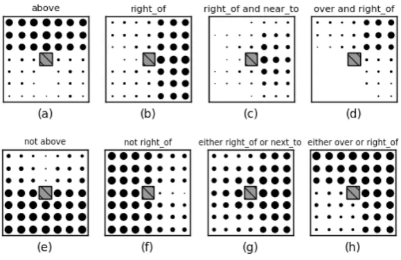
Figure 1: Spatial templates in a 7×7 grid: (a) and (b) are spatial templates for “above” and “right” from (Logan and Sadler, 1996) collected from human judgements. (c-h) are their synthetic compositions. (c) and (d) are intersective-AND compositions of two spatial templates using point-wise multiplication. (e) and (f) represent the negation of (a) and (b) using a complement operation. (g) and (h) are logical-OR compositions of two spatial templates using a point-wise co-multiplication.

in perception to test if the neural language model is able to distinguish them from the words sensitive

to grounding. For example: “{the object|it|the ball}is{spatial phrase} {the object|it|the box}”. The

following additional grammar rules were applied during the generation of the second dataset:

g₁ : (v∗)→[v∗]

g2 : (v∗)→[“it”,“is”,v∗]

g3 : (v∗)→[“it”,“is”,v∗,“the00,“box00]

g₄ : (v∗)→[“the”,“ball”,“is”,v∗,“the00,“box00] g5 : (v∗)→[“the”,“ob ject”,“is”,v∗,“the00,“box00]

(11)

Algorithm 1Synthetic generator

1: n=5

2: gcompositional ={g1,g¬,g∧,g∨} 3: gtextual={g1,g2,g3,g4,g5}

4: procedureSyntheticGenerator(v∗,c,g) 5: f req←n×sˆg(v∗),c

6: for1to f reqdo

7: syntax←choose random(gtextual) 8: text←syntax(g(v∗))

9: Generate(text,c)

In the generated descriptions, words such asand, not, the, box, ball, it, object,andisare not grounded in

locations individually but the phrases they occur in refer to locations on the map.

3

Neural network architecture

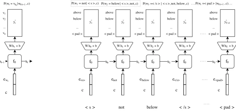
Figure 2: The diagram on the left illustrates the architecture of the model at word/time-steptusing a

vocabulary sizen. On the right, there is an unfolded example how a phrase like “not below” is paired

with a locationcas in (w_1:T,c) and fed as input to the LSTM decoder. In this setup, similar to (Graves, 2013), we train the model to predict the next word in a sequence and the chain of output probabilities is taken to estimate the final probability. The sequence can be cut before reaching the end tag< /s>.

yt = Pr(wt|w1:t−1,c)

ht = fθ(ewt−1;c,ht−1)

ˆyt = softmax(Wht+b)

(12)

where ˆyt is the expected categorical probability at timet, f is a recurrent cell with parametersθ,ewis an

embedding vector for a wordw, andcis an encoded location as a one-hot vector as shown in Figure 2.

The training set in a batch are pairs of word sequences and their corresponding location codes: {(w(i)1:T,c(i))}i∈D where Dis our training dataset. The loss function used is the cross entropy distance

between predicted distribution and targeted distribution or log-loss. The observed true output y(_ti) is

represented with one-hot encodings. The training process can be summarised as follows:

y(_ti) = δ_w(i) t

L(i)(Θ) = −PT_t=+₁1yT(_ti)log(ˆy(_ti))

= −PT_t=+₁1log(ˆy_t(i)(w(_ti)))

(13)

We train the network parameters withAdam stochastic gradient descent (Kingma and Ba, 2014) with

batch normalisation implemented as an optimiser in Keras (Chollet, 2015). On each mini-batch update as (Θb ←Θb−1+AdamS GD(∇ΘL)) the following parameters of the model (Θ) are updated:

{ew}w∈V Embedding vectors for all words

θ Parameters of the RNN cell, composed feature vectors

W,b Parameters of the final dense layer

(14)

3.1 Implementation

We implemented our model in Keras (Chollet, 2015) with TensorFlow (Abadi et al., 2015) as a back-end. All parameters were initialised randomly with Keras recommendations. In the current implementation,

the size of theht, the hidden unit of LSTM, is 15, and the parameters of the RNN cell have a dropout of

0.1. The dropout on embeddings is set to 0.3.

We left-padded descriptionsw1:T0 with a starting tokenw₀ =< s > and right-padded them with a

length ofT +1 as illustrated in Figure 2. The finalyT+1can be either< pad>or< /s>. The length of

the RNN chain has to be of the fixed sizeT +1, the length of the longest possible sentence, in order to

be used with Keras and its implementation on graphic cards.

During each experiment, we trained the model until it reached an over-fitting point with equal training and validation loss.

3.2 From the outputs of the RNN to probabilities of composed descriptions

The decoder architecture of RNNs is normally used as a generator which produces sequences of words or characters from an encoded sequence, e.g. (Cho et al., 2014; Graves, 2013). This can be achieved by applying Equation 1. The decoder predicts the most likely next word in a chain of softmax productions

ˆ

yt. The unfolded RNN in Figure 2 shows how for a sequence of words as input vectors, ˆytare predicted

which represent categorical probabilities for all possible following words at a time step t. For a given

sequence,w1:T =vk1:kt, we estimate the probabilities using Equation 1 as follows:

Pr(wt =vkt|w1:t−1 =vk1:kt,c) = yˆt(vkt)

Pr(w1:T =vk1:kT|c) =

QT

t=1yˆt(vkt)

(15)

The estimated probability is then used to generate spatial templates as in Equation 5. The probabilities

over all possible locations on the mapLfor a given composition of words can be aggregated as follows:

ˆ

Tvk_1:kT0 ={Pr(w1:T0 =vk1:kT0|c)}c∈L (16)

4

Evaluation

We evaluate the learning of composed grounded phrases by examining to what degree the spatial tem-plates produced by the learned model correspond to the original spatial temtem-plates that were used in

gen-erating the training data, how successful is the learning with different kinds of compositions, and what

is the effect of adding distractor words. We ran two experiments, (1) on a simple synthetic dataset

con-taining short phrases where all words are grounded in locations, and (2) on a synthetic dataset generated with five additional grammar rules from Equation 11, introducing words without spatial grounding or distractor words. We test the learning of compositional phrases by training a language model on phrases produced by individual composition types as well as all composition types in both synthetic datasets. A comparison of the predicted spatial templates with the original spatial templates with Spearman’s rank

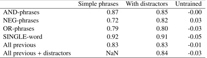
correlation coefficient (Equation 5) in Table 1 shows that there is high correlation between them. We

report the average Spearman’sρand their median p-values for statistical significance.

Simple phrases With distractors Untrained

AND-phrases 0.87 0.85 -0.00

NEG-phrases 0.72 0.82 0.03

OR-phrases 0.79 0.80 -0.03

SINGLE-word 0.92 0.91 -0.05

All previous 0.83 0.83 -0.01

All previous+distractors NaN 0.84 -0.03

Table 1: For each type of compositional phrases we calculate the average Spearman’s rank correlation

coefficient (ρ) between the predicted spatial templates and the templates used to generate the training

data. The median p-value of ρ of all trained models is< 0.001. The columnUntrained indicates the

performance of the model with a random initialisation of weights.

For both Experiment 1 and 2 we created two variations: (1) learning of novel grounded compositions,

hidden from the learner; (2) learning of novel single words from grounded compositions, where propor-tions of single-word instances are omitted from the dataset and their representapropor-tions can only be learned from their occurrence in composed phrases with other words.

In all experiments we hold out 10% of the dataset for validation. In Experiment 1 we iterated the training over 64 epochs using a batch size 8. In Experiment 2, using a batch size 256, we stopped learning iterations before 1024 epochs if the validation loss became equal to the training loss.

4.1 Experiment 1: Learning composition of short phrases

In this experiment the training data is generated for single spatial words, AND-compositions, OR-compositions, and negated phrases without additional distractor words save “and”, “either”, “or”, and “not”.

4.1.1 Learning of novel grounded compositions

The training data contains synthesised samples of all single words and their negations. However, different

proportions of AND-phrases and OR-phrases are removed from the training set to test if the model can

learn unseen composed phrases. Table 2 shows the average of Spearman’s ρcorrelation coefficient for

different portions of held-out phrases. Figure 3 illustrates some predicted novel grounded compositions

where 50% of complex phrases were held out. Theρscores lower than 0.6 may not be trustworthy, e.g.

“above and left of” withρ=0.5 in Figure 3.

Proportions of 90 combinations 10% 20% 30% 40% 50% 60% 70% 80% 90% 100%

AND-phrases 0.84 0.8 0.78 0.76 0.71 0.67 0.64 0.53 0.45 0.29

OR-phrases 0.74 0.73 0.69 0.67 0.56 0.57 0.54 0.38 0.23 -0.23

Table 2: Spearman’sρfor held-out proportions of phrases up to 80% have a median p-value<0.001 and

p-value>0.05 for higher proportions.

Figure 3: The predicted spatial templates are shown on the top and the original spatial templates in the bottom.

The results indicate that the model can produce spatial templates for novel compositions. However, the learning of composed phrases is dependent on the size and the variety of training instances. Some

phrases are more difficult to train than others. For example, OR phrases correspond to regions that are

more spread out across the 48 locations which makes them more difficult to learn, e.g. an extreme case

10% 20% 30% 40%

AND-phrases 0.86 0.8 0.77 0.81

NEG-phrases 0.83 0.64 0.59 0.43

OR-phrases 0.73 0.78 0.68 0.69

SINGLE-word 0.9 0.9 0.84 0.87

Figure 4: The average Spearman’sρfor

dif-ferent proportions of unseen examples. _{Figure 5: The predicted and the original spatial template.}

4.1.2 Learning of novel single words from grounded compositions

In this experiment we omit identical proportions of all description types, thus also single word descrip-tions and negated descripdescrip-tions. In this case, the predicted novel spatial templates are learned solely based on observing these words in combination with other words. As before, we conduct the test with

different sizes of held-out data. The results are shown in Figure 4. When omitting up to 4 single

de-scriptions (right of, over, far from andunder) the average ρon grounded SINGLE-word descriptions

decreases only by 0.05 (from 0.92, Table 1). This means that their grounding is successfully learned from grounded composed expressions. Figure 5 shows a novel learned spatial template for “above”.

4.1.3 Qualitative observations

A qualitative examination of the predicted spatial templates shows that spatial templates with the lowest

ρ are those with no points in space (“right of and left of”) or those with a uniform spread of points

across space (“either far from or next to”) which in our scenario includes a number of training instances

as rules from Section 2.2 were applied to all combinations of spatial templates. We get the highestρwith

compositions such as “over and above”, possibly because the two spatial templates overlap and result in a simplified composed representation.

4.2 Experiment 2: Adding distractor words with no spatial grounding

In Experiment 2 we train and measure the performance of the model on grounded descriptions which also include non-grounded distractor words, for example: “the ball is not left of the box” or “it is above and right of the object”. The words such as “ball”, “object”, “box”, “it” and “is” provide no contribution to the grounded meaning (location). In this dataset the number of possible composed phrases increases from 200 to 1,000. Algorithm 1 in Section 2.2 ensures that in the 1,000 possible phrases the same number of instances is generated as before, now per each of the five permutation rules introducing distractors. The held-out proportions of spatial descriptions are created before Algorithm 1 is applied so permutations including these are not generated.

4.2.1 Learning of novel grounded compositions

Although now the training data includes longer sequences and several distractors which make these compositions harder to learn, the results are only slightly weaker than in Experiment 1 as shown by a comparison of Table 3 with Table 2.

Proportions of 90 combinations 10% 20% 30% 40% 50% 60% 70% 80%

AND-phrases 0.82 0.79 0.75 0.78 0.73 0.69 0.66 0.45

OR-phrases 0.78 0.69 0.67 0.66 0.59 0.59 0.44 0.33

Table 3: The average Spearman’sρwith the median p-value of< 0.001. After 80% of held-out phrase

10% 20% 30% 40%

AND-phrases 0.82 0.60 0.71 0.81

NEG-phrases 0.75 0.66 0.45 0.30

OR-phrases 0.76 0.76 0.71 0.64

SINGLE-word 0.88 0.43 0.73 0.84

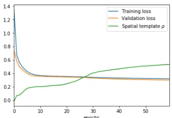
Figure 6: The average Spearman’s correlations

de-composition task Experiment 2. Figure 7: The learning curve for Experiment 3.

4.2.2 Learning of novel single words from grounded compositions

The results of this task on the dataset from Experiment 2 are shown in Figure 6. The ρ are nearly

identical or only slightly lower for SINGLE-words compared to Experiment 1 (Figure 4). There is an

unusual drop inρat 20% of held-out descriptions which requires further investigation. Overall, we can

conclude that the system successfully learned omitted single words from their grounded compositions even with distractor words.

4.3 Experiment 3: How much grounding?

In Experiment 3, we examine how the amount of training corresponds to the groundedness of expressions in spatial templates. In particular, we examine the learning curve across several epochs at which more of the same data is presented incrementally to the learner and how well does the currently learned model corresponds to the target spatial templates. Typically, the performance of the learner at each epoch is es-timated by a loss function, here the cross-entropy (log-loss). We compare the loss at each epoch with the

average Spearman’sρbetween the predicted templates and the original templates for 110 possible

com-binations of descriptions from Experiment 1 (excluding OR-phrases). Here, we only run the experiment

with 20% omission of the dataset. Figure 7 shows how averageρcorresponds to the learning progress.

The figure shows that even after the training and the validation loss are only slightly decreasing between epochs the groundedness is increasing at a higher rate. This can be explained by the fact that the network is not only predicting locations but also sequences of descriptions which adds a further complexity to learning which is reflected in the loss.

5

Conclusion and future work

We have presented a grounded language model with recurrent deep neural networks. The objective of our task was to examine to what extent our neural network architecture can learn a grounded language model that generated the training data and whether a word that is grounded as a part of a phrase can “carry over” its grounding to another phrase not observed in the training data. In our view this is the ultimate test that grounding is compositional. We conduct two learning experiments. In the first experiment we learn a grounded language model where all descriptions in a sequence are grounded. In the subsequent sub-experiments we test the success of the grounded language models where some word compositions are omitted from training. We show that the model is capable of grounding novel compositions and also predicting grounding of single words while only learning from compositions. However, the degree of success, while on overall high, is dependent on the amount of the absent information and the coverage of the training instances. In the second experiment, we add words to our grounded language model

that have no grounding and test whether the system is able to learn different grounding sensitivities of

different words. We show that our language model is capable of recognising the contribution of each

examine grounding related to the log-loss success rate of learning. Overall, we conclude that our deep neural architecture successfully learns grounded spatial descriptions in a way that the learned functions are similar to the ones that generated the data. This is a useful result which points towards the fact that language is compositional both at the level of word sequences and the portions of scenes that they refer to, thus confirming the result in (Dobnik and Åstbom, 2017). In the future work we will focus on the

effects of the varying dataset sizes on the rate of learning and test the learning setup on more complex

perceptual representations (in terms of the expected irregularities) such as images.

References

Abadi, M., A. Agarwal, P. Barham, E. Brevdo, Z. Chen, C. Citro, G. S. Corrado, A. Davis, J. Dean, M. Devin, S. Ghemawat, I. Goodfellow, A. Harp, G. Irving, M. Isard, Y. Jia, R. Jozefowicz, L. Kaiser, M. Kudlur, J. Levenberg, D. Man´e, R. Monga, S. Moore, D. Murray, C. Olah, M. Schuster, J. Shlens, B. Steiner, I. Sutskever, K. Talwar, P. Tucker, V. Vanhoucke, V. Vasudevan, F. Vi´egas, O. Vinyals, P. Warden, M. Wattenberg, M. Wicke, Y. Yu, and X. Zheng (2015). TensorFlow: Large-scale machine learning on heterogeneous systems. Software available from tensorflow.org.

Baroni, M., R. Bernardi, and R. Zamparelli (2014). Frege in space: A program of compositional

distri-butional semantics. LiLT (Linguistic Issues in Language Technology) 9.

Bengio, Y., R. Ducharme, P. Vincent, and C. Jauvin (2003). A neural probabilistic language model. journal of machine learning research 3(Feb), 1137–1155.

Cho, K., B. Van Merri¨enboer, C. Gulcehre, D. Bahdanau, F. Bougares, H. Schwenk, and Y. Bengio (2014). Learning phrase representations using rnn encoder-decoder for statistical machine translation. arXiv preprint arXiv:1406.1078.

Chollet, F. (2015). Keras. https://github.com/fchollet/keras.

Coecke, B., M. Sadrzadeh, and S. Clark (2010). Mathematical foundations for a compositional

distribu-tional model of meaning.arXiv preprint arXiv:1003.4394.

Coventry, K. R., A. Cangelosi, R. Rajapakse, A. Bacon, S. Newstead, D. Joyce, and L. V. Richards (2004). Spatial prepositions and vague quantifiers: Implementing the functional geometric framework. InInternational Conference on Spatial Cognition, pp. 98–110. Springer.

Dobnik, S. (2009, September 4). Teaching mobile robots to use spatial words. Ph. D. thesis, University

of Oxford: Faculty of Linguistics, Philology and Phonetics and The Queen’s College, Oxford, United Kingdom.

Dobnik, S. and A. Åstbom (2017, August 15–17). (Perceptual) grounding as interaction. In V. Petukhova

and Y. Tian (Eds.),Proceedings of Saardial – Semdial 2017: The 21st Workshop on the Semantics and

Pragmatics of Dialogue, Saarbr¨ucken, Germany, pp. 17–26.

Dobnik, S. and R. Cooper (2017). Interfacing language, spatial perception and cognition in Type Theory

with Records.Accepted for Journal of Language Modelling n(n), 1–30.

Gapp, K.-P. (1994, 12-14 September). A computational model of the basic meanings of graded composite

spatial relations in 3D space. InAdvanced geographic data modelling. Spatial data modelling and

query languages for 2D and 3D applications (Proceedings of the AGDM’94), Publications on Geodesy 40, pp. 66–79. Netherlands Geodetic Commission.

Graves, A. (2013). Generating sequences with recurrent neural networks. arXiv preprint

Grice, H. P. (1975). Logic and conversation. In P. Cole and J. Morgan (Eds.),Syntax and Semantics: Speech Acts, Volume 3, pp. 41–58. Academic Press.

Harnad, S. (1990). The symbol grounding problem.Physica D: Nonlinear Phenomena 42(1-3), 335–346.

Herskovits, A. (1986). Language and spatial cognition: an interdisciplinary study of the prepositions in

English. Cambridge: Cambridge University Press.

Hochreiter, S. and J. Schmidhuber (1997). Long short-term memory. Neural computation 9(8), 1735–

1780.

Jøsang, A. and D. McAnally (2005). Multiplication and comultiplication of beliefs.International Journal

of Approximate Reasoning 38(1), 19–51.

Karpathy, A. and L. Fei-Fei (2015). Deep visual-semantic alignments for generating image descriptions. InProceedings of the IEEE Conference on Computer Vision and Pattern Recognition, pp. 3128–3137.

Kingma, D. and J. Ba (2014). Adam: A method for stochastic optimization. arXiv preprint

arXiv:1412.6980.

Kiros, R., R. Salakhutdinov, and R. S. Zemel (2014). Unifying visual-semantic embeddings with

multi-modal neural language models.arXiv preprint arXiv:1411.2539.

Logan, G. D. and D. D. Sadler (1996). A computational analysis of the apprehension of spatial relations.

In P. Bloom, M. A. Peterson, L. Nadel, and M. F. Garrett (Eds.),Language and Space, pp. 493–530.

Cambridge, MA: MIT Press.

Lu, J., C. Xiong, D. Parikh, and R. Socher (2016). Knowing when to look: Adaptive attention via a

visual sentinel for image captioning.arXiv preprint arXiv:1612.01887.

Matuszek, C., N. FitzGerald, L. Zettlemoyer, L. Bo, and D. Fox (2012). A joint model of language and

perception for grounded attribute learning. arXiv preprint arXiv:1206.6423.

McMahan, B. and M. Stone (2015). A bayesian model of grounded color semantics. Transactions of the

Association for Computational Linguistics 3, 103–115.

Mikolov, T., M. Karafi´at, L. Burget, J. Cernock`y, and S. Khudanpur (2010). Recurrent neural network

based language model. InInterspeech, Volume 2, pp. 3.

Mitchell, J. and M. Lapata (2010). Composition in distributional models of semantics. Cognitive

sci-ence 34(8), 1388–1429.

Mnih, A. and G. Hinton (2007). Three new graphical models for statistical language modelling. In Proceedings of the 24th international conference on Machine learning, pp. 641–648. ACM.

Monroe, W., N. D. Goodman, and C. Potts (2016). Learning to generate compositional color descriptions. arXiv preprint arXiv:1606.03821.

Montague, R. (1974). Formal Philosophy: Selected Papers of Richard Montague. New Haven: Yale

University Press.

Ramsey, F. P. (1931). Truth and probability (1926). The foundations of mathematics and other logical

essays, 156–198.

Roy, D. (2005). Semiotic schemas: A framework for grounding language in action and perception. Artificial Intelligence 167(1-2), 170–205.

Roy, D. and N. Mukherjee (2005). Towards situated speech understanding: Visual context priming of

Socher, R., A. Karpathy, Q. V. Le, C. D. Manning, and A. Y. Ng (2014). Grounded compositional

semantics for finding and describing images with sentences.Transactions of the Association for

Com-putational Linguistics 2, 207–218.

Xu, K., J. Ba, R. Kiros, K. Cho, A. C. Courville, R. Salakhutdinov, R. S. Zemel, and Y. Bengio (2015).

Show, attend and tell: Neural image caption generation with visual attention. InICML, Volume 14,