A Joint Many Task Model: Growing a Neural Network for Multiple NLP Tasks

A Joint Many-Task Model:

Growing a Neural Network for Multiple NLP Tasks

Kazuma Hashimoto∗_{, Caiming Xiong}†_{, Yoshimasa Tsuruoka, and Richard Socher} The University of Tokyo

{hassy, tsuruoka}@logos.t.u-tokyo.ac.jp

Salesforce Research

{cxiong, rsocher}@salesforce.com

Abstract

Transfer and multi-task learning have traditionally focused on either a single source-target pair or very few, similar tasks. Ideally, the linguistic levels of mor-phology, syntax and semantics would ben-efit each other by being trained in a sin-gle model. We introduce a joint many-task model together with a strategy for succes-sively growing its depth to solve increas-ingly complex tasks. Higher layers in-clude shortcut connections to lower-level task predictions to reflect linguistic hierar-chies. We use a simple regularization term to allow for optimizing all model weights to improve one task’s loss without exhibit-ing catastrophic interference of the other tasks. Our single end-to-end model ob-tains state-of-the-art or competitive results on five different tasks from tagging, pars-ing, relatedness, and entailment tasks.

1 Introduction

The potential for leveraging multiple levels of representation has been demonstrated in various ways in the field of Natural Language Processing (NLP). For example, Part-Of-Speech (POS) tags are used for syntactic parsers. The parsers are used to improve higher-level tasks, such as natural lan-guage inference (Chen et al.,2016) and machine translation (Eriguchi et al.,2016). These systems are often pipelines and not trained end-to-end.

Deep NLP models have yet shown benefits from predicting many increasingly complex tasks each at a successively deeper layer. Existing models often ignore linguistic hierarchies by predicting

∗_{Work was done while the first author was an intern at}

Salesforce Research.

†_{Corresponding author.}

CHUNK

POS DEP

Relatedness encoder

Relatedness Entailment

encoder

Entailment

word representation

Sentence1

CHUNK

POS DEP

Relatedness encoder Entailment

encoder

word representation

Sentence2

semantic level

syntactic level

wor

[image:1.595.320.520.225.400.2]

d level

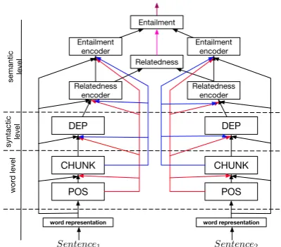
Figure 1: Overview of the joint many-task model predicting different linguistic outputs at succes-sively deeper layers.

different tasks either entirely separately or at the same depth (Collobert et al.,2011).

We introduce a Joint Many-Task (JMT) model, outlined in Figure 1, which predicts increasingly complex NLP tasks at successively deeper lay-ers. Unlike traditional pipeline systems, our sin-gle JMT model can be trained end-to-end for POS tagging, chunking, dependency parsing, semantic relatedness, and textual entailment, by consider-ing lconsider-inguistic hierarchies. We propose an adaptive training and regularization strategy to grow this model in its depth. With the help of this strat-egy we avoid catastrophic interference between the tasks. Our model is motivated bySøgaard and Goldberg(2016) who showed that predicting two different tasks is more accurate when performed in different layers than in the same layer (Collobert et al., 2011). Experimental results show that our single model achieves competitive results for all of the five different tasks, demonstrating that

ing linguistic hierarchies is more important than handling different tasks in the same layer.

2 The Joint Many-Task Model

This section describes the inference procedure of our model, beginning at the lowest level and work-ing our way to higher layers and more complex tasks; our model handles the five different tasks in the order of POS tagging, chunking, dependency parsing, semantic relatedness, and textual entail-ment, by considering linguistic hierarchies. The POS tags are used for chunking, and the chunking tags are used for dependency parsing (Attardi and DellOrletta,2008). Tai et al. (2015) have shown that dependencies improve the relatedness task. The relatedness and entailment tasks are closely related to each other. If the semantic relatedness between two sentences is very low, they are un-likely to entail each other. Based on this obser-vation, we make use of the information from the relatedness task for improving the entailment task.

2.1 Word Representations

For each wordwtin the input sentencesof length

L, we use two types of embeddings.

Word embeddings: We use Skip-gram (Mikolov et al.,2013) to train word embeddings.

Character embeddings: Character n-gram em-beddings are trained by the same Skip-gram ob-jective. We construct the charactern-gram vocab-ulary in the training data and assign an ding for each entry. The final character embed-ding is the average of theuniquecharactern-gram embeddings ofwt. For example, the charactern

-grams (n = 1,2,3) of the word “Cat” are {C, a, t, #B#C, Ca, at, t#E#, #B#Ca, Cat, at#E#}, where “#B#” and “#E#” represent the beginning and the end of each word, respectively. Using the char-acter embeddings efficiently provides morpholog-ical features. Each word is subsequently repre-sented asxt, the concatenation of its

correspond-ing word and character embeddcorrespond-ings shared across the tasks.1

2.2 Word-Level Task: POS Tagging

The first layer of the model is a bi-directional

LSTM (Graves and Schmidhuber,2005;

Hochre-iter and Schmidhuber,1997) whose hidden states 1_{Bojanowski et al.(2017) previously proposed to train the}

charactern-gram embeddings by the Skip-gram objective.

are used to predict POS tags. We use the follow-ing Long Short-Term Memory (LSTM) units for the forward direction:

it = σ(Wigt+bi), ft=σ(Wfgt+bf),

ut = tanh (Wugt+bu),

ct = itut+ftct−1, (1)

ot = σ(Wogt+bo), ht=ottanh (ct),

where we define the inputgt asgt = [→−ht−1;xt],

i.e. the concatenation of the previous hidden state and the word representation ofwt. The backward

pass is expanded in the same way, but a different set of weights are used.

For predicting the POS tag of wt, we use the

concatenation of the forward and backward states in a one-layer bi-LSTM layer corresponding to the

t-th word:ht= [−→ht;←−ht]. Then eachht(1≤t≤

L)is fed into a standardsoftmaxclassifier with a single ReLUlayer which outputs the probability vectory(1)_{for each of the POS tags.}

2.3 Word-Level Task: Chunking

Chunking is also a word-level classification task which assigns a chunking tag (B-NP,I-VP, etc.) for each word. The tag specifies the region of ma-jor phrases (e.g., noun phrases) in the sentence.

Chunking is performed in the second bi-LSTM layer on top of the POS layer. When stacking the bi-LSTM layers, we use Eq. (1) with input

g(2)_t = [h(2)_t−1;h(1)_t ;xt;y(tpos)], where h(1)t is the

hidden state of the first (POS) layer. We define the weighted label embeddingy(_tpos)as follows:

y_t(pos) =XC

j=1

p(y(1)_t =j|h(1)_t )`(j), (2)

whereC is the number of the POS tags,p(y(1)_t =

j|h(1)_t )is the probability value that the j-th POS tag is assigned towt, and `(j)is the

correspond-ing label embeddcorrespond-ing. The probability values are predicted by the POS layer, and thus no gold POS tags are needed. This output embedding is simi-lar to theK-best POS tag feature which has been shown to be effective in syntactic tasks (Andor et al., 2016; Alberti et al., 2015). For predict-ing the chunkpredict-ing tags, we employ the same strat-egy as POS tagging by using the concatenated bi-directional hidden states h(2)_t = [−→h_t(2);←−h(2)_t ] in

the chunking layer. We also use a singleReLU

2.4 Syntactic Task: Dependency Parsing

Dependency parsing identifies syntactic relations (such as an adjective modifying a noun) between word pairs in a sentence. We use the third bi-LSTM layer to classify relations between all pairs of words. The input vector for the LSTM in-cludes hidden states, word representations, and the label embeddings for the two previous tasks:

g(3)_t = [h(3)_t−1;h(2)_t ;xt; (yt(pos)+y(tchk))], where we

computed the chunking vector in a similar fashion as the POS vector in Eq. (2).

We predict the parent node (head) for each

word. Then a dependency label is predicted for each child-parent pair. This approach is related to Dozat and Manning (2017) and Zhang et al.

(2017), where the main difference is that our model works on a multi-task framework. To pre-dict the parent node ofwt, we define a matching

function betweenwtand the candidates of the

par-ent node asm(t, j) =h(3)_t ·(Wdh(3)j ), whereWd

is a parameter matrix. For the root, we define

h(3)_L+1 = r as a parameterized vector. To com-pute the probability thatwj (or the root node) is

the parent ofwt, the scores are normalized:

p(j|h(3)_t ) = P_L+1exp (m(t, j))

k=1,k6=texp (m(t, k))

. (3)

The dependency labels are predicted using

[h(3)_t ;h(3)_j ] as input to a softmax classifier with a singleReLUlayer. We greedily select the par-ent node and the dependency label for each word. When the parsing result is not a well-formed tree, we apply the first-order Eisner’s algorithm (Eisner,

1996) to obtain a well-formed tree from it.

2.5 Semantic Task: Semantic relatedness

The next two tasks model the semantic relation-ships between two input sentences. The first task measures the semantic relatedness between two sentences. The output is a real-valued relatedness score for the input sentence pair. The second task is textual entailment, which requires one to deter-mine whether a premise sentence entails a hypoth-esis sentence. There are typically three classes: entailment, contradiction, and neutral. We use the fourth and fifth bi-LSTM layer for the relatedness and entailment task, respectively.

Now it is required to obtain the sentence-level representation rather than the word-level represen-tation h(4)_t used in the first three tasks. We com-pute the sentence-level representationh(4)s as the

element-wise maximum values across all of the word-level representations in the fourth layer:

h(4)s = max

h(4)₁ , h(4)₂ , . . . , h(4)_L . (4)

This max-pooling technique has proven effective in text classification tasks (Lai et al.,2015).

To model the semantic relatedness between s

and s0_{, we follow Tai et al. (2015). The feature} vector for representing the semantic relatedness is computed as follows:

d1(s, s0) =hh(4)s −h(4)_s0 ;h(4)s h(4)_s0

i , (5)

where h(4)s −h(4)_s0 is the absolute values of the

element-wise subtraction, and h(4)s h(4)_s0 is the

element-wise multiplication. Thend1(s, s0)is fed

into a softmax classifier with a single Maxout

hidden layer (Goodfellow et al., 2013) to output a relatedness score (from 1 to 5 in our case).

2.6 Semantic Task: Textual entailment

For entailment classification, we also use the max-pooling technique as in the semantic relatedness task. To classify the premise-hypothesis pair

(s, s0_{) into one of the three classes, we} com-pute the feature vectord2(s, s0) as in Eq. (5) ex-cept that we do not use the absolute values of the element-wise subtraction, because we need to identify which is the premise (or hypothesis). Thend2(s, s0)is fed into asoftmaxclassifier.

To use the output from the relatedness layer di-rectly, we use the label embeddings for the related-ness task. More concretely, we compute the class label embeddings for the semantic relatedness task similar to Eq. (2). The final feature vectors that are concatenated and fed into the entailment classifier are the weighted relatedness label embedding and the feature vectord2(s, s0). We use threeMaxout hidden layers before the classifier.

3 Training the JMT Model

The model is trained jointly over all datasets. Dur-ing each epoch, the optimization iterates over each full training dataset in the same order as the corre-sponding tasks described in the modeling section.

3.1 Pre-Training Word Representations

We pre-train word embeddings using the

et al., 2013). We also pre-train the character n -gram embeddings using Skip--gram.2 _{The only} dif-ference is that each input word embedding is re-placed with its corresponding average charactern -gram embedding described in Section2.1. These embeddings are fine-tuned during the model train-ing. We denote the embedding parameters asθe.

3.2 Training the POS Layer

Let θPOS = (WPOS, bPOS, θe) denote the set of

model parameters associated with the POS layer, where WPOS is the set of the weight matrices in the first bi-LSTM and the classifier, andbPOS is the set of the bias vectors. The objective function to optimizeθPOSis defined as follows:

J1(θPOS) =−

X

s

X

t

logp(y_t(1)=α|h(1)_t )

+λkWPOSk2+δkθe−θ0ek2,

(6)

wherep(y_t(1) = αwt|h(1)t )is the probability value

that the correct labelαis assigned towtin the

sen-tences,λkWPOSk2is the L2-norm regularization term, andλis a hyperparameter.

We call the second regularization term δkθe −

θ0

ek2 a successive regularization term. The

suc-cessive regularization is based on the idea that we do not want the model to forget the information learned for the other tasks. In the case of POS tagging, the regularization is applied toθe, andθ0e

is the embedding parameter after training the final task in the top-most layer at the previous training epoch.δis a hyperparameter.

3.3 Training the Chunking Layer

The objective function is defined as follows:

J2(θchk) =−

X

s

X

t

logp(y(2)_t =α|h(2)_t )

+λkWchkk2+δkθPOS−θPOS0 k2,

(7)

which is similar to that of POS tagging, andθchkis (Wchk, bchk, EPOS, θe), where Wchk andbchk are the weight and bias parameters including those in

θPOS, and EPOS is the set of the POS label em-beddings. θ0

POS is the one after training the POS layer at the current training epoch.

2_{The training code and the pre-trained embeddings}

are available at https://github.com/hassyGo/ charNgram2vec.

3.4 Training the Dependency Layer

The objective function is defined as follows:

J3(θdep) =−

X

s

X

t

logp(α|h(3)_t )p(β|h(3)_t , h(3)_α )

+λ(kWdepk2+kWdk2) +δkθchk−θchk0 k2,

(8)

where p(α|h(3)_t ) is the probability value

as-signed to the correct parent node α for wt,

and p(β|h(3)_t , h(3)α ) is the probability value

as-signed to the correct dependency label β for

the child-parent pair (wt, α). θdep is defined as (Wdep, bdep, Wd, r, EPOS, Echk, θe), where Wdep and bdep are the weight and bias parameters in-cluding those in θchk, and Echk is the set of the chunking label embeddings.

3.5 Training the Relatedness Layer

FollowingTai et al.(2015), the objective function is defined as follows:

J4(θrel) =

X

(s,s0₎

KLpˆ(s, s0)p(h(4)_s , h(4)_s0 )

+λkWrelk2+δkθdep−θ0depk2,

(9)

wherepˆ(s, s0_{)is the gold distribution over the} de-fined relatedness scores, p(h(4)s , h(4)_s0 ) is the

pre-dicted distribution given the the sentence repre-sentations, andKLpˆ(s, s0_)p(h(4)_{s , h}(4)

s0 )

is the KL-divergence between the two distributions. θrel is defined as(Wrel, brel, EPOS, Echk, θe).

3.6 Training the Entailment Layer

The objective function is defined as follows:

J5(θent) =−

X

(s,s0₎

logp(y₍(5)_s,s0₎ =α|h(5)_s , h(5)_s0 )

+λkWentk2+δkθrel−θ0relk2, (10)

where p(y(5)_(s,s0₎ = α|h(5)s , h(5)_s0 ) is the

probabil-ity value that the correct label α is assigned to the premise-hypothesis pair(s, s0_).θ

entis defined as(Went, bent, EPOS, Echk, Erel, θe), whereErelis the set of the relatedness label embeddings.

4 Related Work

designed to handle single tasks, or some of them

are designed as general-purpose models (Kumar

et al.,2016;Sutskever et al.,2014) but applied to different tasks independently.

For handling multiple NLP tasks, multi-task learning models with deep neural networks have been proposed (Collobert et al.,2011;Luong et al.,

2016), and more recently Søgaard and Goldberg

(2016) have suggested that using different layers for different tasks is more effective than using the same layer in jointly learning closely-related tasks, such as POS tagging and chunking. However, the number of tasks was limited or they have very sim-ilar task settings like word-level tagging, and it was not clear how lower-level tasks could be also improved by combining higher-level tasks.

More related to our work,Godwin et al.(2016)

also followed Søgaard and Goldberg (2016) to

jointly learn POS tagging, chunking, and

lan-guage modeling, and Zhang and Weiss (2016)

have shown that it is effective to jointly learn POS tagging and dependency parsing by sharing inter-nal representations. In the field of relation extrac-tion, Miwa and Bansal (2016) proposed a joint learning model for entity detection and relation ex-traction. All of them suggest the importance of multi-task learning, and we investigate the poten-tial of handling different types of NLP tasks rather than closely-related ones in a single hierarchical deep model.

In the field of computer vision, some trans-fer and multi-task learning approaches have also been proposed (Li and Hoiem,2016;Misra et al.,

2016). For example,Misra et al.(2016) proposed a multi-task learning model to handle different tasks. However, they assume that each data sam-ple has annotations for the different tasks, and do not explicitly consider task hierarchies.

Recently, Rusu et al. (2016) have proposed a progressive neural network model to handle mul-tiple reinforcement learning tasks, such as Atari games. Like our JMT model, their model is also successively trained according to different tasks using different layers called columns in their pa-per. In their model, once the first task is com-pleted, the model parameters for the first task are fixed, and then the second task is handled with new model parameters. Therefore, accuracy of the pre-viously trained tasks is never improved. In NLP tasks, multi-task learning has the potential to im-prove not only higher-level tasks, but also

lower-level tasks. Rather than fixing the pre-trained model parameters, our successive regularization allows our model to continuously train the lower-level tasks without significant accuracy drops.

5 Experimental Settings

5.1 Datasets

POS tagging:To train the POS tagging layer, we used the Wall Street Journal (WSJ) portion of Penn Treebank, and followed the standard split for the training (Section 0-18), development (Section 19-21), and test (Section 22-24) sets. The evaluation metric is the word-level accuracy.

Chunking: For chunking, we also used the WSJ corpus, and followed the standard split for the training (Section 15-18) and test (Section 20) sets as in the CoNLL 2000 shared task. We used Sec-tion 19 as the development set and employed the IOBES tagging scheme. The evaluation metric is the F1 score defined in the shared task.

Dependency parsing:We also used the WSJ cor-pus for dependency parsing, and followed the stan-dard split for the training (Section 2-21), devel-opment (Section 22), and test (Section 23) sets. We obtained Stanford style dependencies using the version 3.3.0 of the Stanford converter. The evalu-ation metrics are the Unlabeled Attachment Score (UAS) and the Labeled Attachment Score (LAS), and punctuations are excluded for the evaluation.

Semantic relatedness: For the semantic related-ness task, we used the SICK dataset (Marelli et al.,

2014), and followed the standard split for the train-ing, development, and test sets. The evaluation metric is the Mean Squared Error (MSE) between the gold and predicted scores.

Textual entailment: For textual entailment, we also used the SICK dataset and exactly the same data split as the semantic relatedness dataset. The evaluation metric is the accuracy.

5.2 Training Details

the number of bi-LSTM layers involved in each task, and3.0is the maximum value. We applied our successive regularization to our model, along with L2-norm regularization and dropout ( Srivas-tava et al.,2014). More details are summarized in the supplemental material.

6 Results and Discussion

Table 1 shows our results on the test sets of the five tasks.3 _{The column “Single” shows the} re-sults of handling each task separately using single-layer bi-LSTMs, and the column “JMTall” shows the results of our JMT model. The single task set-tings only use the annotations of their own tasks. For example, when handling dependency parsing as a single task, the POS and chunking tags arenot

used. We can see that all results of the five tasks are improved in our JMT model, which shows that our JMT model can handle the five different tasks in a single model. Our JMT model allows us to access arbitrary information learned from the dif-ferent tasks. If we want to use the model just as a POS tagger, we can use only first bi-LSTM layer.

Table 1 also shows the results of five subsets of the different tasks. For example, in the case of “JMTABC”, only the first three layers of the bi-LSTMs are used to handle the three tasks. In the case of “JMTDE”, only the top two layers are used as a two-layer bi-LSTM by omitting all in-formation from the first three layers. The results of the closely-related tasks (“AB”, “ABC”, and “DE”) show that our JMT model improves both of the high-level and low-level tasks. The results of “JMTCD” and “JMTCE” show that the parsing task can be improved by the semantic tasks.

It should be noted that in our analysis on the greedy parsing results of the “JMTABC” setting, we have found that more than 95% are well-formed dependency trees on the development set. In the 1,700 sentences of the development data, 11 results have multiple root notes, 11 results have no root nodes, and 61 results have cycles. These 83 parsing results are converted into well-formed trees by Eisner’s algorithm, and the accuracy does not significantly change (UAS: 94.52%→94.53%,

LAS: 92.61%→92.62%).

3_{In chunking evaluation, we only show the results of}

“Sin-gle” and “JMTAB” because the sentences for chunking

eval-uation overlap the training data for dependency parsing.

6.1 Comparison with Published Results POS tagging Table2 shows the results of POS tagging, and our JMT model achieves the score close to the state-of-the-art results. The best result to date has been achieved by Ling et al. (2015), which uses character-based LSTMs. Incorporat-ing the character-based encoders into our JMT model would be an interesting direction, but we have shown that the simple pre-trained character

n-gram embeddings lead to the promising result.

Chunking Table 3 shows the results of chunk-ing, and our JMT model achieves the state-of-the-art result. Søgaard and Goldberg(2016) proposed to jointly learn POS tagging and chunking in dif-ferent layers, but they only showed improvement for chunking. By contrast, our results show that the low-level tasks are also improved.

Dependency parsing Table4shows the results of dependency parsing by using only the WSJ cor-pus in terms of the dependency annotations.4 _{It is} notable that our simple greedy dependency parser

outperforms the model in Andor et al. (2016)

which is based on beam search with global infor-mation. The result suggests that the bi-LSTMs ef-ficiently capture global information necessary for dependency parsing. Moreover, our single task result already achieves high accuracy without the POS and chunking information. The best result to date has been achieved by the model propsoed in

Dozat and Manning(2017), which uses higher di-mensional representations than ours and proposes a more sophisticated attention mechanism called

biaffine attention. It should be promising to incor-porate their attention mechanism into our parsing component.

Semantic relatedness Table5shows the results of the semantic relatedness task, and our JMT model achieves the state-of-the-art result. The re-sult of “JMTDE” is already better than the previous state-of-the-art results. Both ofZhou et al.(2016) andTai et al.(2015) explicitly used syntactic trees, andZhou et al.(2016) relied on attention mecha-nisms. However, our method uses the simple max-pooling strategy, which suggests that it is worth 4_{Choe and Charniak (2016) employed a tri-training}

Single JMTall JMTAB JMTABC JMTDE JMTCD JMTCE

A↑ POS 97.45 97.55 97.52 97.54 n/a n/a n/a

B↑ Chunking 95.02 n/a 95.77 n/a n/a n/a n/a

C↑ Dependency UAS_{Dependency LAS} 93.35_91.42 94.67_92.90 n/a_n/a 94.71_92.92 n/a_{n/a 91.62}93.53 93.57_91.69

D↓ Relatedness 0.247 0.233 n/a n/a 0.238 0.251 n/a

[image:7.595.108.487.62.135.2]

E↑ Entailment 81.8 86.2 n/a n/a 86.8 n/a 82.4

Table 1: Test set results for the five tasks. In the relatedness task, the lower scores are better.

Method Acc.↑

JMTall 97.55

Ling et al.(2015) 97.78

Kumar et al.(2016) 97.56

Ma and Hovy(2016) 97.55

Søgaard(2011) 97.50

Collobert et al.(2011) 97.29

Tsuruoka et al.(2011) 97.28

Toutanova et al.(2003) 97.27

Table 2: POS tagging results.

Method F1↑

JMTAB 95.77

Single 95.02

Søgaard and Goldberg(2016) 95.56

Suzuki and Isozaki(2008) 95.15

Collobert et al.(2011) 94.32

Kudo and Matsumoto(2001) 93.91

Tsuruoka et al.(2011) 93.81

Table 3: Chunking results.

Method UAS↑ LAS↑

JMTall 94.67 92.90

Single 93.35 91.42

Dozat and Manning(2017) 95.74 94.08

Andor et al.(2016) 94.61 92.79

Alberti et al.(2015) 94.23 92.36

Zhang et al.(2017) 94.10 91.90

Weiss et al.(2015) 93.99 92.05

Dyer et al.(2015) 93.10 90.90

[image:7.595.129.220.284.326.2]

Bohnet(2010) 92.88 90.71

Table 4: Dependency results.

Method MSE↓

JMTall 0.233

JMTDE 0.238

Zhou et al.(2016) 0.243

[image:7.595.325.505.364.407.2]

Tai et al.(2015) 0.253

Table 5: Semantic relatedness results.

Method Acc.↑

JMTall 86.2

JMTDE 86.8

Yin et al.(2016) 86.2

Lai and Hockenmaier(2014) 84.6

Table 6: Textual entailment results.

JMTall w/o SC w/o LE w/o SC&LE

POS 97.88 97.79 97.85 97.87

Chunking 97.59 97.08 97.40 97.33

Dependency UAS 94.51 94.52 94.09 94.04

Dependency LAS 92.60 92.62 92.14 92.03

Relatedness 0.236 0.698 0.261 0.765

Entailment 84.6 75.0 81.6 71.2

Table 7: Effectiveness of the Shortcut Connections (SC) and the Label Embeddings (LE).

investigating such simple methods before develop-ing complex methods for simple tasks. Currently, our JMT model does not explicitly use the learned dependency structures, and thus the explicit use of the output from the dependency layer should be an interesting direction of future work.

Textual entailment Table6shows the results of textual entailment, and our JMT model achieves the the-art result. The previous state-of-the-art result in Yin et al. (2016) relied on at-tention mechanisms and dataset-specific data pre-processing and features. Again, our simple max-pooling strategy achieves the state-of-the-art result boosted by the joint training. These results show the importance of jointly handling related tasks.

6.2 Analysis on the Model Architectures

We investigate the effectiveness of our model in detail. All of the results shown in this section are the development set results.

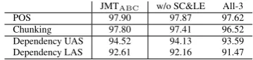
JMTABC w/o SC&LE All-3

POS 97.90 97.87 97.62

Chunking 97.80 97.41 96.52

Dependency UAS 94.52 94.13 93.59

Dependency LAS 92.61 92.16 91.47

Table 8: Effectiveness of using different layers for different tasks.

Shortcut connections Our JMT model feeds the word representations into all of the bi-LSTM lay-ers, which is called the shortcut connection. Ta-ble7shows the results of “JMTall” with and out the shortcut connections. The results with-out the shortcut connections are shown in the col-umn of “w/o SC”. These results clearly show that the importance of the shortcut connections, and in particular, the semantic tasks in the higher layers strongly rely on the shortcut connections. That is, simply stacking the LSTM layers is not sufficient to handle a variety of NLP tasks in a single model. In the supplementary material, it is qualitatively shown how the shortcut connections work in our model.

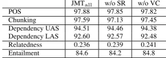
[image:7.595.76.285.364.424.2]

JMTall w/o SR w/o VC

POS 97.88 97.85 97.82

Chunking 97.59 97.13 97.45

Dependency UAS 94.51 94.46 94.38

Dependency LAS 92.60 92.57 92.48

Relatedness 0.236 0.239 0.241

[image:8.595.351.481.62.122.2]

Entailment 84.6 84.2 84.8

Table 9: Effectiveness of the Successive Regular-ization (SR) and the Vertical Connections (VC).

JMTall Random

POS 97.88 97.83

Chunking 97.59 97.71

Dependency UAS 94.51 94.66

Dependency LAS 92.60 92.80

Relatedness 0.236 0.298

[image:8.595.98.262.63.121.2]

Entailment 84.6 83.2

Table 10: Effects of the order of training.

model. The results in the column of “w/o SC&LE” are the ones without both of the shortcut connec-tions and the label embeddings.

Different layers for different tasks Table 8

shows the results of our “JMTABC” setting and that of not using the shortcut connections and the label embeddings (“w/o SC&LE”) as in Table7. In addition, in the column of “All-3”, we show the results of using the highest (i.e., the third) layer for all of the three tasks without any shortcut connec-tions and label embeddings, and thus the two set-tings “w/o SC&LE” and “All-3” require exactly the same number of the model parameters. The “All-3” setting is similar to the multi-task model ofCollobert et al.(2011) in that task-specific out-put layers are used but most of the model param-eters are shared. The results show that using the same layers for the three different tasks hampers the effectiveness of our JMT model, and the de-sign of the model is much more important than the number of the model parameters.

Successive regularization In Table 9, the col-umn of “w/o SR” shows the results of omitting the successive regularization terms described in Sec-tion3. We can see that the accuracy of chunking is improved by the successive regularization, while other results are not affected so much. The chunk-ing dataset used here is relatively small compared with other low-level tasks, POS tagging and de-pendency parsing. Thus, these results suggest that the successive regularization is effective when dataset sizes are imbalanced.

Vertical connections We investigated our JMT results without using the vertical connections in

Single Single+

POS 97.52

Chunking 95.65 96.08

Dependency UAS 93.38 93.88

Dependency LAS 91.37 91.83

Relatedness 0.239 0.665

Entailment 83.8 66.4

Table 11: Effects of depth for thesingletasks.

Single W&C Only W

POS 97.52 96.26

Chunking 95.65 94.92

Dependency UAS 93.38 92.90

[image:8.595.352.477.157.203.2]

Dependency LAS 91.37 90.44

Table 12: Effects of the character embeddings.

the five-layer bi-LSTMs. More concretely, when constructing the input vectors gt, we do not use

the bi-LSTM hidden states of the previous lay-ers. Table 9 also shows the JMTall results with and without the vertical connections. As shown in the column of “w/o VC”, we observed the compet-itive results. Therefore, in the target tasks used in our model, sharing the word representations and the output label embeddings is more effective than just stacking the bi-LSTM layers.

Order of training Our JMT model iterates the training process in the order described in Sec-tion3. Our hypothesis is that it is important to start from the lower-level tasks and gradually move to the higher-level tasks. Table10shows the results of training our model by randomly shuffling the order of the tasks for each epoch in the column of “Random”. We see that the scores of the semantic tasks drop by the random strategy. In our prelimi-nary experiments, we have found that constructing the mini-batch samples from different tasks also hampers the effectiveness of our model, which also supports our hypothesis.

Depth The single task settings shown in Table1

[image:8.595.115.248.171.232.2]

mak-ing the models complex only for smak-ingle tasks.

Character n-gram embeddings Finally, Ta-ble12shows the results for the three single tasks with and without the pre-trained charactern-gram embeddings. The column of “W&C” corresponds to using both of the word and character n-gram embeddings, and that of “Only W” corresponds to using only the word embeddings. These re-sults clearly show that jointly using the pre-trained word and charactern-gram embeddings is helpful in improving the results. The pre-training of the charactern-gram embeddings is also effective; for example, without the pre-training, the POS accu-racy drops from 97.52% to 97.38% and the chunk-ing accuracy drops from 95.65% to 95.14%.

6.3 Discussion

Training strategies In our JMT model, it is not obvious when to stop the training while trying to maximize the scores of all the five tasks. We fo-cused on maximizing the accuracy of dependency parsing on the development data in our experi-ments. However, the sizes of the training data are different across the different tasks; for exam-ple, the semantic tasks include only 4,500 sen-tence pairs, and the dependency parsing dataset includes 39,832 sentences with word-level anno-tations. Thus, in general, dependency parsing requires more training epochs than the semantic tasks, but currently, our model trains all of the tasks for the same training epochs. The same strat-egy for decreasing the learning rate is also shared across all the different tasks, although our growing gradient clipping method described in Section5.2

helps improve the results. Indeed, we observed that better scores of the semantic tasks can be achieved before the accuracy of dependency pars-ing reaches the best score. Developpars-ing a method for achieving the best scores for all of the tasks at the same time is important future work.

More tasks Our JMT model has the potential of handling more tasks than the five tasks used in our experiments; examples include entity

de-tection and relation extraction as in Miwa and

Bansal(2016) as well as language modeling ( God-win et al.,2016). It is also a promising direction to train each task for multiple domains by focus-ing on domain adaptation (Søgaard and Goldberg,

2016). In particular, incorporating language mod-eling tasks provides an opportunity to use large text data. Such large text data was used in our

experiments to pre-train the word and charactern -gram embeddings. However, it would be prefer-able to efficiently use it for improving the entire model.

Task-oriented learning of low-level tasks Each task in our JMT model is supervised by its cor-responding dataset. However, it would be possi-ble to learn low-level tasks by optimizing high-level tasks, because the model parameters of the low-level tasks can be directly modified by learn-ing the high-level tasks. One example has

al-ready been presented inHashimoto and Tsuruoka

(2017), where our JMT model is extended to learn-ing task-oriented latent graph structures of sen-tences by training our dependency parsing com-ponent according to a neural machine translation objective.

7 Conclusion

We presented a joint many-task model to handle multiple NLP tasks with growing depth in a sin-gle end-to-end model. Our model is successively trained by considering linguistic hierarchies, di-rectly feeding word representations into all lay-ers, explicitly using low-level predictions, and ap-plying successive regularization. In experiments on five NLP tasks, our single model achieves the state-of-the-art or competitive results on chunk-ing, dependency parschunk-ing, semantic relatedness, and textual entailment.

Acknowledgments

We thank the anonymous reviewers and the Sales-force Research team members for their fruitful comments and discussions.

References

Chris Alberti, David Weiss, Greg Coppola, and Slav Petrov. 2015. Improved Transition-Based Parsing and Tagging with Neural Networks. In Proceed-ings of the 2015 Conference on Empirical Methods in Natural Language Processing, pages 1354–1359. Daniel Andor, Chris Alberti, David Weiss, Aliaksei Severyn, Alessandro Presta, Kuzman Ganchev, Slav Petrov, and Michael Collins. 2016. Globally Nor-malized Transition-Based Neural Networks. In Pro-ceedings of the 54th Annual Meeting of the Associa-tion for ComputaAssocia-tional Linguistics (Volume 1: Long Papers), pages 2442–2452.

Bernd Bohnet. 2010. Top Accuracy and Fast Depen-dency Parsing is not a Contradiction. In Proceed-ings of the 23rd International Conference on Com-putational Linguistics, pages 89–97.

Piotr Bojanowski, Edouard Grave, Armand Joulin, and Tomas Mikolov. 2017. Enriching Word Vectors with Subword Information. Transactions of the Associa-tion for ComputaAssocia-tional Linguistics, 5:135–146. Qian Chen, Xiaodan Zhu, Zhenhua Ling, Si Wei, and

Hui Jiang. 2016. Enhancing and Combining Se-quential and Tree LSTM for Natural Language In-ference.arXiv, cs.CL 1609.06038.

Do Kook Choe and Eugene Charniak. 2016. Parsing as Language Modeling. InProceedings of the 2016 Conference on Empirical Methods in Natural Lan-guage Processing, pages 2331–2336.

Ronan Collobert, Jason Weston, Leon Bottou, Michael Karlen nad Koray Kavukcuoglu, and Pavel Kuksa. 2011. Natural Language Processing (Al-most) from Scratch. Journal of Machine Learning Research, 12:2493–2537.

Timothy Dozat and Christopher D. Manning. 2017. Deep Biaffine Attention for Neural Dependency Parsing. In Proceedings of the 5th International Conference on Learning Representations.

Chris Dyer, Miguel Ballesteros, Wang Ling, Austin Matthews, and Noah A. Smith. 2015. Transition-Based Dependency Parsing with Stack Long Short-Term Memory. InProceedings of the 53rd Annual Meeting of the Association for Computational Lin-guistics and the 7th International Joint Conference on Natural Language Processing (Volume 1: Long Papers), pages 334–343.

Jason Eisner. 1996. Efficient Normal-Form Parsing for Combinatory Categorial Grammar. InProceedings of the 34th Annual Meeting of the Association for Computational Linguistics, pages 79–86.

Akiko Eriguchi, Kazuma Hashimoto, and Yoshimasa Tsuruoka. 2016. Tree-to-Sequence Attentional Neu-ral Machine Translation. InProceedings of the 54th Annual Meeting of the Association for Computa-tional Linguistics (Volume 1: Long Papers), pages 823–833.

Jonathan Godwin, Pontus Stenetorp, and Sebastian Riedel. 2016. Deep Semi-Supervised Learning with Linguistically Motivated Sequence Labeling Task Hierarchies.arXiv, cs.CL 1612.09113.

Ian J. Goodfellow, David Warde-Farley, Mehdi Mirza, Aaron Courville, and Yoshua Bengio. 2013. Max-out Networks. In Proceedings of The 30th Inter-national Conference on Machine Learning, pages 1319–1327.

Alex Graves and Jurgen Schmidhuber. 2005. Frame-wise Phoneme Classification with Bidirectional LSTM and Other Neural Network Architectures.

Neural Networks, 18(5):602–610.

Kazuma Hashimoto and Yoshimasa Tsuruoka. 2017. Neural Machine Translation with Source-Side La-tent Graph Parsing. InProceedings of the 2017 Con-ference on Empirical Methods in Natural Language Processing. To appear.

Sepp Hochreiter and Jurgen Schmidhuber. 1997. Long short-term memory. Neural Computation, 9(8):1735–1780.

Taku Kudo and Yuji Matsumoto. 2001. Chunking with Support Vector Machines. In Proceedings of the Second Meeting of the North American Chapter of the Association for Computational Linguistics.

Ankit Kumar, Ozan Irsoy, Peter Ondruska, Mohit Iyyer, James Bradbury, Ishaan Gulrajani, Victor Zhong, Romain Paulus, and Richard Socher. 2016. Ask Me Anything: Dynamic Memory Networks for Natural Language Processing. In Proceedings of The 33rd International Conference on Machine Learning, pages 1378–1387.

Adhiguna Kuncoro, Miguel Ballesteros, Lingpeng Kong, Chris Dyer, Graham Neubig, and Noah A. Smith. 2017. What Do Recurrent Neural Network Grammars Learn About Syntax? In Proceedings of the 15th Conference of the European Chapter of the Association for Computational Linguistics, pages 1249–1258.

Alice Lai and Julia Hockenmaier. 2014. Illinois-LH: A Denotational and Distributional Approach to Se-mantics. In Proceedings of the 8th International Workshop on Semantic Evaluation, pages 329–334.

Siwei Lai, Liheng Xu, Kang Liu, and Jun Zhao. 2015. Recurrent Convolutional Neural Networks for Text Classification. InProceedings of the Twenty-Ninth AAAI Conference on Artificial Intelligence, pages 2267–2273.

Zhizhong Li and Derek Hoiem. 2016. Learning with-out Forgetting. CoRR, abs/1606.09282.

Wang Ling, Chris Dyer, Alan W Black, Isabel Tran-coso, Ramon Fermandez, Silvio Amir, Luis Marujo, and Tiago Luis. 2015. Finding Function in Form: Compositional Character Models for Open Vocab-ulary Word Representation. In Proceedings of the 2015 Conference on Empirical Methods in Natural Language Processing, pages 1520–1530.

Minh-Thang Luong, Ilya Sutskever, Quoc V. Le, Oriol Vinyals, and Lukasz Kaiser. 2016. Multi-task Se-quence to SeSe-quence Learning. InProceedings of the 4th International Conference on Learning Represen-tations.

Marco Marelli, Luisa Bentivogli, Marco Baroni, Raf-faella Bernardi, Stefano Menini, and Roberto Zam-parelli. 2014. SemEval-2014 Task 1: Evaluation of Compositional Distributional Semantic Models on Full Sentences through Semantic Relatedness and Textual Entailment. In Proceedings of the 8th In-ternational Workshop on Semantic Evaluation (Se-mEval 2014), pages 1–8.

Tomas Mikolov, Ilya Sutskever, Kai Chen, Greg S Cor-rado, and Jeff Dean. 2013. Distributed Representa-tions of Words and Phrases and their Composition-ality. InAdvances in Neural Information Processing Systems 26, pages 3111–3119.

Ishan Misra, Abhinav Shrivastava, Abhinav Gupta, and Martial Hebert. 2016. Cross-stitch Networks for Multi-task Learning.CoRR, abs/1604.03539. Makoto Miwa and Mohit Bansal. 2016. End-to-End

Relation Extraction using LSTMs on Sequences and Tree Structures. In Proceedings of the 54th An-nual Meeting of the Association for Computational Linguistics (Volume 1: Long Papers), pages 1105– 1116.

Andrei A. Rusu, Neil C. Rabinowitz, Guillaume Des-jardins, Hubert Soyer, James Kirkpatrick, Koray Kavukcuoglu, Razvan Pascanu, and Raia Hadsell. 2016. Progressive Neural Networks. CoRR, abs/1606.04671.

Anders Søgaard. 2011. Semi-supervised condensed nearest neighbor for part-of-speech tagging. In Pro-ceedings of the 49th Annual Meeting of the Associ-ation for ComputAssoci-ational Linguistics: Human Lan-guage Technologies, pages 48–52.

Anders Søgaard and Yoav Goldberg. 2016. Deep multi-task learning with low level tasks supervised at lower layers. InProceedings of the 54th Annual Meeting of the Association for Computational Lin-guistics (Volume 2: Short Papers), pages 231–235. Nitish Srivastava, Geoffrey Hinton, Alex Krizhevsky,

Ilya Sutskever, and Ruslan Salakhutdinov. 2014. Dropout: A Simple Way to Prevent Neural Networks from Overfitting. Journal of Machine Learning Re-search, 15:1929–1958.

Ilya Sutskever, Oriol Vinyals, and Quoc V Le. 2014. Sequence to Sequence Learning with Neural Net-works. InAdvances in Neural Information Process-ing Systems 27, pages 3104–3112.

Jun Suzuki and Hideki Isozaki. 2008. Semi-Supervised Sequential Labeling and Segmentation Using Giga-Word Scale Unlabeled Data. InProceedings of the 46th Annual Meeting of the Association for Com-putational Linguistics: Human Language Technolo-gies, pages 665–673.

Kai Sheng Tai, Richard Socher, and Christopher D. Manning. 2015. Improved Semantic Representa-tions From Tree-Structured Long Short-Term Mem-ory Networks. InProceedings of the 53rd Annual

Meeting of the Association for Computational Lin-guistics and the 7th International Joint Conference on Natural Language Processing (Volume 1: Long Papers), pages 1556–1566.

Kristina Toutanova, Dan Klein, Christopher D Man-ning, and Yoram Singer. 2003. Feature-Rich Part-of-Speech Tagging with a Cyclic Dependency Net-work. In Proceedings of the 2003 Human Lan-guage Technology Conference of the North Ameri-can Chapter of the Association for Computational Linguistics, pages 173–180.

Yoshimasa Tsuruoka, Yusuke Miyao, and Jun’ichi Kazama. 2011. Learning with Lookahead: Can History-Based Models Rival Globally Optimized Models? In Proceedings of the Fifteenth Confer-ence on Computational Natural Language Learning, pages 238–246.

David Weiss, Chris Alberti, Michael Collins, and Slav Petrov. 2015. Structured Training for Neural Net-work Transition-Based Parsing. InProceedings of the 53rd Annual Meeting of the Association for Computational Linguistics and the 7th International Joint Conference on Natural Language Processing (Volume 1: Long Papers), pages 323–333.

Wenpeng Yin, Hinrich Schtze, Bing Xiang, and Bowen Zhou. 2016. ABCNN: Attention-Based Convolu-tional Neural Network for Modeling Sentence Pairs.

Transactions of the Association for Computational Linguistics, 4:259–272.

Xingxing Zhang, Jianpeng Cheng, and Mirella Lapata. 2017. Dependency Parsing as Head Selection. In

Proceedings of the 15th Conference of the European Chapter of the Association for Computational Lin-guistics, pages 665–676.

Yuan Zhang and David Weiss. 2016. Stack-propagation: Improved Representation Learning for Syntax. In Proceedings of the 54th Annual Meet-ing of the Association for Computational LMeet-inguistics (Volume 1: Long Papers), pages 1557–1566. Yao Zhou, Cong Liu, and Yan Pan. 2016. Modelling