Magnetothermoelastic Problem of a Half-Space Subjected to
Moving Heat Source and Moving Load
S.K. Bhullar and J.L.Wegner
Abstract-This paper is concerned to study temperature distribution, thermal stresses and displacement components for a magnetothermoelastic problem of a half-space subjected to (i) moving heat source and (ii) moving load. Classical Dynamical Coupled, Lord-Shulman and Green Lindsay theories of thermoelasticity are used for mathematical analysis. It is found that the Lord-Shulman theory is more pronounced than coupled theory and Green Lindsay theories. Numerical computations have been performed for computing temperature, stresses and displacement for these theories. The results obtained using these theories are compared and depicted graphically.
Keywords: displacement, temperature field, moving heat source, moving load.
Nomenclature
C-D Classical Dynamical Coupled L-S Lord-Shulman theory G-L Green Lindsay theory
f
Arbitrary functionν
Velocity of motionu
G
Displacementh
Surface heat transfer coefficientt
Timek
Thermal conductivity,
0t
t
1 Relaxation timesT Absolute temperature
0
T
Reference temperature chosen so that1 | 0 |T −T <<
e
Dilatation,ε
kkj i
e Components of strain deviator
i
u
Components of displacement vectorE
C
Components of displacement vectorManuscript submitted on December 3, 2009. S.K Bhullar and J. L. Wegner
Department of Mechanical Engineering, University of Victoria, PO Box 3055, Victoria, B.C. Canada V8W 3P6
E-mail: [email protected] and [email protected]
2 c
0 0
1
ε
μ
2 0 c
ρ
μ
λ
+
2
Greek notation
j i
σ
Stress componentsμ
λ
, Lam constantsρ
Density0
μ
Magnetic permability b Electric permabilityi
α
Coefficient of linear thermal expansion
γ
(
)
i
α
μ
λ
23 +
ε
E
C
ρ
γ
α
22 0
1
c
a
+
0
α
αβ
2
η
0K
C
Eρ
β
2 22 2 0
c
c
Subscript
0
E
j i
1. Introduction
relaxation time. This modified theory is known as the generalized theory of thermoelasticity. Later, Green and Lindsay [2] developed a more general theory of thermoelasticity, in which Fourier.s law of heat conduction is unchanged,
whereas the classical energy equation and the stress-strain temperature relations are modified by introducing two constitutive constants having dimensions of time. In the last five decades another domain has been developed, which investigates the interaction between the strain and electromagnetic fields. This discipline is called magnetoelasticity. The problem of interaction between the elastic or thermoelastic field and the electromagnetic field has been a research topic for a number of investigations in recent years because of it’s utilitarian aspects in various branches of science and technology, like geophysics for understanding the effect of the Earth’s magnetic field on seismic waves, damping of acoustic waves in a magnetic field, emissions at electromagnetic radiation from nuclear devices, development of a highly sensitive super conducting magnetometer, electrical power engineering, optics and plasma physics. A comprehensive review of the earlier contribution to the subject can be found in [3]. The contribution of some authors who had worked in this field is presented in [4-11]. The other studies performed is a coupled magnetothermoelastic problem in elastic half space [12], transient generalized magnetothermoelastic waves in a rotating half-space [13] and a coupled magnetothermoelastic problem in a perfectly conducting elastic half-space with thermal relaxation [14], magnetothermoelastic waves induced by a thermal shock in a infinitely conducting elastic half space [15] and generation of generalized magneto thermoelastic waves by thermal shock in a perfectly conducting half-space[16]. Recently, relaxation effects on thermal shock problems in an elastic half-space of generalized magneto thermoelasticity are stidied in [17].
In the present paper we have formulated a two-dimensional magnetothermoelastic problem of a half- space subjected to moving heat source and moving load to study temperature field, thermal stresses and displacement components.
2. Theory
Following Othman [17], for generalized thermoelasticity with two relaxation times, the linearized equations in non- dimensional form of electrodynamics in slowly moving medium and the non-vanishing stress components are given by
(
)
(
)
(
1
)
1
, 1 , 2
, 2 , , 2
u
t
v
u
u
o x x
xy yy
xx
α
θ
θ
β
β
β
=
+
−
−
+
+
(
)
(
)
(
2
)
1
, 1 2
, , 2 , 2
v
t
v
v
u
o y y
xx yy xy
α
θ
θ
β
β
β
=
+
−
+
+
−
) 3 ( 2
2 2 2 2
e t o t t
t o t t
⎟ ⎟ ⎠ ⎞ ⎜
⎜ ⎝ ⎛
∂ ∂ + ∂
∂ +
⎟ ⎟ ⎠ ⎞ ⎜
⎜ ⎝ ⎛
∂ ∂ + ∂
∂ = ∇
ε
θ θ
(
)
) 4 ( 1
2
1 2
, 2 , 2 0
θ β
β β
σ
⎟⎟ ⎠ ⎞ ⎜⎜
⎝ ⎛
∂ ∂ + −
− + =
t t
v
ux y
x x
(
)
) 5 ( 1
2
1 2
, 2 0 , 2
θ β
β β
σ
⎟⎟ ⎠ ⎞ ⎜⎜
⎝ ⎛
∂ ∂ + −
+ −
=
t t
u
ux y
yy
) 6 ( ,
,x x xy = u +v σ
) 7 (
, ,x vy
u
e= +
.
,
,
2
,
,
1
,
1
,
2 2 2 2 2 0 2 2 0 2
0
2 0 0 2 0 0 0 2 2 2 0 2
0
ρ
μ
β
ρ
μ
λ
ρ
μ
ε
μ
α
αβ
α
=
=
+
+
=
=
=
+
=
=
c
c
c
a
c
H
a
c
c
a
0
t
andt
1 are thermal relaxation times and other symbols have their usual meanings. In order to discuss the results from different theories of thermoelasticity,we shall take for: C-D theory,
t
0=
t
1=
0
;L-S theory,
t
0=
0
,
t
1≠
0
;G-L theory,
t
0≠
0
,
t
1≠
0
.,
,
,
,
,
,
,
0 0 0 1 0 1 0 0
0 0
0 0 0
0 0
0 0
t
t
t
t
t
t
v
T
c
v
u
T
c
u
y
c
y
x
c
x
η
η
η
η
ρ
η
ρ
η
η
=
′
=
′
=
′
=
′
=
′
=
′
=
′
.
,
,
00 0
K
C
T
T
T
Eij ij
ρ
η
θ
μ
σ
σ
′
=
=
−
=
where, primes denote dimensional variables. If we introduce the function
ϕ
defined by,) 8 (
θ
ϕ
=e−Equations (1) and (2) take the form
(
)
(9)1
2 2 2 1 2 2
2
t t
t ∂
∂ − ∇ − ∇ = ∂
∂ ϕ θ ϕ
α
θ
The heat conduction equation given by(3) can be written as
(
)
[
]
(10)2 2
2θ θ +εθ +ϕ
⎟⎟ ⎠ ⎞ ⎜⎜
⎝ ⎛
∂ ∂ + ∂
∂ = ∇
t t
t o
and the stress components given by (4) - (6) are written as
) 11 ( 2
1
, 2 0
1 2 2 0
y x
x
v t t
− +
⎥ ⎦ ⎤ ⎢
⎣ ⎡
⎟⎟ ⎠ ⎞ ⎜⎜
⎝ ⎛
∂ ∂ + − =
ϕ β
θ β
β σ
) 12 ( 2
1
, 2 0
1 2 2 0
x yy
u t t
− +
⎥ ⎦ ⎤ ⎢
⎣ ⎡
⎟⎟ ⎠ ⎞ ⎜⎜
⎝ ⎛
∂ ∂ + − =
ϕ β
θ β
β σ
)
13
(
, ,y x
xy
=
u
+
v
σ
We change the co-ordinate system moving with input by shifting the origin to the position of input
(
)
) 14 ( , , ,
2 2 2 2 2 1
0 0
y x
t t y y t p x c x
′′ ∂
∂ + ′′ ∂
∂ = ∇
′ = ′′ ′ = ′′ ′ − ′ = ′′ η
where ,
0 c
v
p= is the dimensionless loading
speed and the co-ordinates x′′and y′′ move in positive direction with speed p. It follows from (14) that we may use the relation
) 15 ( x
p
t ∂ ′′
∂ − = ′ ∂
∂
to eliminate time derivatives. In terms of the moving co-ordinates given by (14) , (1) and (2) together with (7) and (8) become
(
)
(
)
(
16
)
1
, 2 ,
1 , 2
, , , 2
xx o xx x
xx yy x
u
p
pt
u
u
α
θ
θ
β
ϕ
θ
β
=
−
−
+
+
+
−
(
)
(
)
(
17
)
1
, 2 ,
1 , 2
, , , 2
xx o yy y
xx yy y
v
p
pt
v
v
α
θ
θ
β
ϕ
θ
β
=
−
−
+
+
+
−
Equations (9)-(10) together with relation (15), after omitting the primes on x and y are as follows:
) 18 ( 1
2 2 2
2 1 2 2
2
x p
x pt x
∂ ∂ −
⎟⎟ ⎠ ⎞ ⎜⎜
⎝ ⎛
∂ ∂ ∇ + ∇ = ∂
∂
ϕ
θ ϕ
α θ
(
)
[
]
(19)2 2 2 2
ϕ θ ε θ θ
+ + ×
⎟⎟ ⎠ ⎞ ⎜⎜
⎝ ⎛
∂ ∂ +
∂ ∂ − = ∇
x t p x
p o
To obtain the expressions for θ,ϕ,u,v andσij let us assume that
[
]
( )
[
]
( )
(
)
(20)exp
, , , , , , , ,
, 0 0 0 0 0
Dy ax
y v
u y
x v
u ij ij
− ×
=
ι
σ
ϕ
θ
σ
ϕ
θ
where, D is the (complex) frequency and a is the wave number in the x- direction and D is unknown quantity. Inserting (20) into (18) and (19) to obtain:
[
]
( )
(
)
[
2 2]
0( )
(21)1 2 2
0 2 2 2 2
y a p apt a D
y a p a D
θ α ι ϕ α
+ −
− =
+ −
( )
[
(
2 2)
(
1)
1]
0( )
(22) 01ϕ y D a ε ω θ y
εω = − − +
Eliminating θ0
( )
y from equations (21)-(22), we obtain[
2]
0( )
0 (23)2 1
4− − =
y a D a
D θ
where,
(
1)
12 2 2
1
2
a
αω
p
1
ε
ιε
apt
ω
a
=
+
+
+
+
(
)(
)
(
1)
2 1 2 2
1 4
2
a
a
1
p
a
1
apt
a
=
+
ω
−
α
+
εω
+
ι
ap a p
t
ι
ω
=− 2 2 −0 1
Equation (23) can be factorized as
(
)(
)
[
]
0( )
0 (24)2 2 2 2 1
2 − − =
y k D k
D θ
where,
3 2 2 2
2 ,
1
=
a
+
ω
±
ω
k
(
)
[
1]
12 2
2 1
2
1
α
ε
ιεα
ω
ω
= p a + + + pt4 2 2 2
3
ω
α
p aThe solution of (23) is written as
(
)
(25)exp 1
2
1
0 ax k y
i i − =
∑
=ι
θ
θ
where
θ
iare parameters depending upona
. Substituting equation (25) in (21) and we get:(
)
(
)
∑
=−
×
⎥
⎦
⎤
⎢
⎣
⎡
+
−
+
−
=
2 1 2 2 2 2 2 2 1 2 2 0)
26
(
exp
i i i i iy
k
ax
a
p
a
k
a
p
apt
a
k
ι
θ
α
α
ι
ϕ
Now, (16) and (17) together with (20) become as follows:
(
)
(
)
(
)
0
(
27
)
1
0 1 2 2 0 2 0 2 2 0 2 2=
+
−
−
+
+
−
θ
β
ι
ϕ
β
ι
α
pt
a
a
a
u
a
p
a
D
(
)
(
)
(
1
)
0
(
28
)
1
0 1 2 0 2 0 2 2 0 2 2=
+
+
−
+
+
−
θ
β
ι
ϕ
β
ι
α
D
pt
a
D
a
v
a
p
a
D
Substituting (25) - (26) in (27) (28), we get
(
)(
)
(
)
(
)
(29)exp 1 1
2
1 2 2
1 2 2 2 2 2 2 1 2 2 2 2 2 0 y k ax a pt a a p a k a p apt a k ia m k u i i i i i i − × ⎪ ⎭ ⎪ ⎬ ⎫ ⎪ ⎩ ⎪ ⎨ ⎧ + + + − + − − − − =
∑
= ι θ β ι α α ι β(
)(
)
(
)
(
)
∑
= − × ⎥ ⎥ ⎥ ⎦ ⎤ ⎢ ⎢ ⎢ ⎣ ⎡ − − + − + − − − = 21 1 2
2 2 2 2 2 2 1 2 2 2 2 2 0 ) 30 ( exp 1 1 1 i i i i i i y k ax apt a p a k a p apt a k m k v ι θ β ι α α ι β
where, m=a2 +
α
0a2p2In terms of the moving co-ordinates (14) and by making use of relation (15) the stress components given by (11)-(13) become as follows ) 31 ( 2 1 , 2 0 1 2 2 0 y x x v x pt − + ⎥ ⎦ ⎤ ⎢ ⎣ ⎡ ⎟⎟ ⎠ ⎞ ⎜⎜ ⎝ ⎛ ∂ ∂ − − = ϕ β θ β β σ ) 32 ( 2 1 , 2 0 1 2 2 0 x yy u x pt − + ⎥ ⎦ ⎤ ⎢ ⎣ ⎡ ⎟⎟ ⎠ ⎞ ⎜⎜ ⎝ ⎛ ∂ ∂ − − = ϕ β θ β β σ ) 33 ( ,
,y x xy= u +v σ
Upon using (20), (25), (26) and (29) into equations (31)-(33), we get
( ) ( ) ) 34 ( exp 2 1 2 2 2 2 2 2 2 2 1 2 2 1 2 2 2 1 2 2 2 2 2 2 2 2 2 2 2 1 1 1 0 1 0 0 y k ax i a p a k a p apt a k apt m k k apt a p a k a p apt a k i i i i i i i i xx − × ∑ = ⎪ ⎪ ⎪ ⎪ ⎪ ⎪ ⎭ ⎪⎪ ⎪ ⎪ ⎪ ⎪ ⎬ ⎫ ⎪ ⎪ ⎪ ⎪ ⎪ ⎪ ⎩ ⎪⎪ ⎪ ⎪ ⎪ ⎪ ⎨ ⎧ ⎥ ⎥ ⎥ ⎥ ⎥ ⎦ ⎤ ⎢ ⎢ ⎢ ⎢ ⎢ ⎣ ⎡ + − ⎟ ⎠ ⎞ ⎜ ⎝ ⎛ + ⎟ ⎠ ⎞ ⎜ ⎝ ⎛ − ⎟ ⎠ ⎞ ⎜ ⎝ ⎛ − − ⎟ ⎠ ⎞ ⎜ ⎝ ⎛ − − × − − ⎥ ⎥ ⎥ ⎥ ⎥ ⎦ ⎤ ⎢ ⎢ ⎢ ⎢ ⎢ ⎣ ⎡ − − + + − + ⎟ ⎠ ⎞ ⎜ ⎝ ⎛ − = ι θ α α ι β β ι ι β β α α ι β σ ( )
( ) (35)
exp 2 1 2 2 2 2 2 2 2 2 1 2 2 1 2 2 2 1 2 2 2 2 2 2 2 2 2 2 2 1 1 1 0 1 0 0 y k ax i a p a k a p apt a k apt m k a apt a p a k a p apt a k i i i i i i i yy − × ∑ = ⎪ ⎪ ⎪ ⎪ ⎪ ⎪ ⎭ ⎪⎪ ⎪ ⎪ ⎪ ⎪ ⎬ ⎫ ⎪ ⎪ ⎪ ⎪ ⎪ ⎪ ⎩ ⎪⎪ ⎪ ⎪ ⎪ ⎪ ⎨ ⎧ ⎥ ⎥ ⎥ ⎥ ⎥ ⎦ ⎤ ⎢ ⎢ ⎢ ⎢ ⎢ ⎣ ⎡ + − ⎟ ⎠ ⎞ ⎜ ⎝ ⎛ + ⎟ ⎠ ⎞ ⎜ ⎝ ⎛ − ⎟ ⎠ ⎞ ⎜ ⎝ ⎛ − − ⎟ ⎠ ⎞ ⎜ ⎝ ⎛ + − × − − ⎥ ⎥ ⎥ ⎥ ⎥ ⎦ ⎤ ⎢ ⎢ ⎢ ⎢ ⎢ ⎣ ⎡ − − + + − + ⎟ ⎠ ⎞ ⎜ ⎝ ⎛ − = ι θ α α ι β β ι ι ι β β α α ι β σ ( )
( ) (36)
exp 2 2 2 2 2 2 2 2 1 2 2 1 2 2 2 2 2 2 1 1 2 2 2 2 2 2 2 2 2 2 2 2 2 2 1 1 2 1 1 0 1 0 0 y k ax a p a k a p apt a k apt m k k m k ak i apt a p a k a p apt a k m k k i i i i i i i i i i i i xy − × ⎥ ⎥ ⎥ ⎥ ⎥ ⎦ ⎤ ⎢ ⎢ ⎢ ⎢ ⎢ ⎣ ⎡ + − ⎟ ⎠ ⎞ ⎜ ⎝ ⎛ + ⎟ ⎠ ⎞ ⎜ ⎝ ⎛ − ⎟ ⎠ ⎞ ⎜ ⎝ ⎛ − + ⎟ ⎠ ⎞ ⎜ ⎝ ⎛ + − × − − − ∑ = ⎥ ⎥ ⎥ ⎥ ⎥ ⎦ ⎤ ⎢ ⎢ ⎢ ⎢ ⎢ ⎣ ⎡ − − + + − + ⎟ ⎠ ⎞ ⎜ ⎝ ⎛ − − =
∑
= ι θ α α ι β β ι ι ι β β α α ι β σ Problem IConsider a homogeneous isotropic thermoelastic solid occupying the region
∞ < < ∞ − ∞ < < ∞ −
≥ x z
y 0, ,
of the xy-plane and displacement
u
G
=
(
u
,
v
,
0
)
and the temperature T are function of x,y
where, h is the surface heat transfer coefficient and f is arbitrary function and be the velocity of motion of heat source. Equations (37) together with (25) and(36) gives following expression:
(
)
exp( )
(38)exp 2 1 1 2 1 ax a y k ax i k i
i
ι
ι
θ
∑
∑
= = = − ( )( ) 0(39) exp 2 1 2 2 2 2 2 2 2 2 1 2 2 1 2 2 1 2 2 2 2 2 2 2 2 2 2 2 2 2 2 1 1 1 0 1 0 0 = × ∑ = ⎪ ⎪ ⎪ ⎪ ⎪ ⎪ ⎪ ⎪ ⎭ ⎪ ⎪ ⎪ ⎪ ⎪ ⎪ ⎪ ⎪ ⎬ ⎫ ⎪ ⎪ ⎪ ⎪ ⎪ ⎪ ⎪ ⎪ ⎩ ⎪ ⎪ ⎪ ⎪ ⎪ ⎪ ⎪ ⎪ ⎨ ⎧ ⎥ ⎥ ⎥ ⎥ ⎥ ⎦ ⎤ ⎢ ⎢ ⎢ ⎢ ⎢ ⎣ ⎡ + − ⎟ ⎠ ⎞ ⎜ ⎝ ⎛ + ⎟ ⎠ ⎞ ⎜ ⎝ ⎛ − ⎟ ⎠ ⎞ ⎜ ⎝ ⎛ − + ⎟ ⎠ ⎞ ⎜ ⎝ ⎛ + − × − − ⎥ ⎥ ⎥ ⎥ ⎥ ⎦ ⎤ ⎢ ⎢ ⎢ ⎢ ⎢ ⎣ ⎡ − − + + − + ⎟ ⎠ ⎞ ⎜ ⎝ ⎛ − − = ax i a p a k a p apt a k apt m k ak apt a p a k a p apt a k m k k i i i i i i i i xy ι θ α α ι β β ι ι ι β β α α ι β σ
(
)
exp( )
0 (40)2 1 = +
∑
= ax h k i ii
θ
ι
Where,
( )
( )
2 2 1exp
)
(
and
exp
)
(
1
x
x
f
dx
ax
x
f
a
i k−
=
=
∫
=ι
π
22 21 21 13 2 22 131 , , a a
a a a a + − = ∇ ∇ − = ∇ = θ θ
(
)
(
2)
13 12
11 exp
1 ,
1 a b x t
a
a ν
π − −
= = =
(
)
(
)(
)
(
)(
)
(
)
⎥⎥ ⎥ ⎦ ⎤ ⎢ ⎢ ⎢ ⎣ ⎡ − − + − + − − − + ⎥ ⎥ ⎥ ⎦ ⎤ ⎢ ⎢ ⎢ ⎣ ⎡ + − + − − − + − = 2 1 2 2 2 2 1 2 2 1 2 2 1 2 2 2 1 1 2 2 2 2 1 2 2 1 2 2 1 2 2 2 1 2 2 1 2 1 21 1 1 1 β ι α α ι β ι α α ι β β ι apt a p a k a p apt a k m k k a a p a k a p apt a k ia a pt a m k k a(
)
(
)(
)
(
)(
)
(
)
⎥⎥ ⎥ ⎦ ⎤ ⎢ ⎢ ⎢ ⎣ ⎡ − − + − + − − − + ⎥ ⎥ ⎥ ⎦ ⎤ ⎢ ⎢ ⎢ ⎣ ⎡ + − + − − − + − = 2 1 2 2 2 2 2 2 2 1 2 2 2 2 2 2 2 1 2 2 2 2 2 2 2 1 2 2 2 2 2 2 1 2 2 2 2 2 22 1 1 1 β ι α α ι β ι α α ι β β ι apt a p a k a p apt a k m k k a a p a k a p apt a k ia a pt a m k k a 0 23 = a Problem IIConsider a homogeneous isotropic thermoelastic solid occupying the region
∞ < < ∞ − ∞ < < ∞ −
≥ x z
y 0, , of the
xy-plane which is subjected to moving load with following boundary conditions,
(
x,y,t)
g(
x t)
(41)yy ν
σ = −
(
x,y,t)
=0 (42)xy σ ) 43 ( 0 = + ∂
∂θ θ
h y
(
)
( )
exp( )
(44) exp 2 1 2 2 2 2 2 2 2 2 1 2 2 1 2 2 2 1 2 2 2 2 2 2 2 2 2 2 2 2 1 1 1 1 0 1 0∑
= = × ∑ = ⎪ ⎪ ⎪ ⎪ ⎪ ⎪ ⎭ ⎪ ⎪ ⎪ ⎪ ⎪ ⎪ ⎬ ⎫ ⎪ ⎪ ⎪ ⎪ ⎪ ⎪ ⎩ ⎪ ⎪ ⎪ ⎪ ⎪ ⎪ ⎨ ⎧ ⎥ ⎥ ⎥ ⎥ ⎥ ⎦ ⎤ ⎢ ⎢ ⎢ ⎢ ⎢ ⎣ ⎡ + − ⎟ ⎠ ⎞ ⎜ ⎝ ⎛ + ⎟ ⎠ ⎞ ⎜ ⎝ ⎛ − ⎟ ⎠ ⎞ ⎜ ⎝ ⎛ − − ⎟ ⎠ ⎞ ⎜ ⎝ ⎛ + − × − − ⎥ ⎥ ⎥ ⎥ ⎥ ⎦ ⎤ ⎢ ⎢ ⎢ ⎢ ⎢ ⎣ ⎡ − − + + − + ⎟ ⎠ ⎞ ⎜ ⎝ ⎛ − k i i i i i i ax ax i a p a k a p apt a k apt m k a apt a p a k a p apt a k ι ι θ α α ι β β ι ι ι β β α α ι β(
)
( )
0 (45) exp 2 1 2 2 2 2 2 2 2 2 1 2 2 1 2 2 1 2 2 2 2 2 2 2 2 2 2 2 2 2 2 1 1 1 0 1 0 = × ∑ = ⎪ ⎪ ⎪ ⎪ ⎪ ⎪ ⎪ ⎪ ⎭ ⎪ ⎪ ⎪ ⎪ ⎪ ⎪ ⎪ ⎪ ⎬ ⎫ ⎪ ⎪ ⎪ ⎪ ⎪ ⎪ ⎪ ⎪ ⎩ ⎪ ⎪ ⎪ ⎪ ⎪ ⎪ ⎪ ⎪ ⎨ ⎧ ⎥ ⎥ ⎥ ⎥ ⎥ ⎦ ⎤ ⎢ ⎢ ⎢ ⎢ ⎢ ⎣ ⎡ + − ⎟ ⎠ ⎞ ⎜ ⎝ ⎛ + ⎟ ⎠ ⎞ ⎜ ⎝ ⎛ − ⎟ ⎠ ⎞ ⎜ ⎝ ⎛ − + ⎟ ⎠ ⎞ ⎜ ⎝ ⎛ + − × − − ⎥ ⎥ ⎥ ⎥ ⎥ ⎦ ⎤ ⎢ ⎢ ⎢ ⎢ ⎢ ⎣ ⎡ − − + + − + ⎟ ⎠ ⎞ ⎜ ⎝ ⎛ − − ax i a p a k a p apt a k apt m k ak apt a p a k a p apt a k m k k i i i i i i i i ι θ α α ι β β ι ι ι β β α α ι β(
)
exp( )
0 (46)2 1 = +
∑
= ax h k i ii
θ
ι
where,
( )
( )
22 1 exp ) ( and exp ) ( 1 x x g dx ax x g b i k − = =
∫
=ι
π
22 11 12 21
21 13 2
22 13
1
,
,
a
a
a
a
a
a
a
a
′
′
+
′
′
−
=
∇′
∇′
′
′
−
=
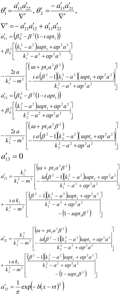
′
∇′
′
′
=
′
θ
θ
(
)
(
)
(
)
(
)
(
)(
)(
)
⎥ ⎥ ⎥
⎦ ⎤
⎢ ⎢ ⎢
⎣ ⎡
+ −
+ −
− −
+
− −
⎥ ⎦ ⎤ ⎢
⎣ ⎡
+ −
+ −
+
− − = ′
2 2 2 2 1
2 2 1 2 2 1 2
2 2 1 2
2 1
2 2 2 2
2 2 1 2 2 1 2 0
1 2
2 0 11
1 2
1
a p a k
a p apt a k a
a pt a
m k
a
a p a k
a p apt a k
apt a
i
α
α ι β
ι
β ι
ι
α α ι β
ι β β
(
)
(
)
(
)
(
)
(
)(
)(
)
⎥ ⎥ ⎥
⎦ ⎤
⎢ ⎢ ⎢
⎣ ⎡
+ −
+ −
− −
+
− −
⎥ ⎦ ⎤ ⎢
⎣ ⎡
+ −
+ −
+
− − = ′
2 2 2 2 2
2 2 1 2 2 2 2
2 2 1 2
2 2
2 2 2 2 2
2 2 1 2 2 2 2 0
1 2
2 0 12
1 2
1
a p a k
a p apt a k a
a pt a
m k
a
a p a k
a p apt a k
apt a
α
α ι β
ι
β ι
ι
α α ι β
ι β β
0
13
′
=
a
(
)
(
)(
)
(
)(
)
(
)
⎥⎥⎥
⎦ ⎤
⎢ ⎢ ⎢
⎣ ⎡
− −
+ −
+ −
−
− +
⎥ ⎥ ⎥
⎦ ⎤
⎢ ⎢ ⎢
⎣ ⎡
+ −
+ −
− −
+
− = ′
2 1
2 2 2 2 1
2 2 1 2 2 1 2
2 2
1
2 2 2 2 1
2 2 1 2 2 1 2
2 2 1
2 2 1
2 1 21
1 1
1
β ι α
α ι β
ι
α α ι β
β ι
apt a p a k
a p apt a k
m k
k a
a p a k
a p apt a k ia
a pt a
m k
k a
i
(
)
(
)(
)
(
)(
)
(
)
⎥⎥⎥
⎦ ⎤
⎢ ⎢ ⎢
⎣ ⎡
− −
+ −
+ −
−
− +
⎥ ⎥ ⎥
⎦ ⎤
⎢ ⎢ ⎢
⎣ ⎡
+ −
+ −
− −
+
− = ′
2 1
2 2 2 2 2
2 2 1 2 2 2 2
2 2 2
1
2 2 2 2 2
2 2 1 2 2 2 2
2 2 1
2 2 2
2 2 22
1 1
1
β ι α
α ι β
ι
α α ι β
β ι
apt a p a k
a p apt a k
m k
k a
a p a k
a p apt a k ia
a pt a
m k
k a
(
)
(
2)
23 exp 1
t x b
a ν
π − −
= ′
3. Numerical calculations and Conclusion
In order to study the temperature field, thermal stresses and displacement components, we have computed them for a specific model. The material chosen for numerical calculation is Copper. The physical data for such material in SI units is,
.
01
.
2
,
5
.
3
,
0168
.
0
,
/
381
,
/
10
398
.
0
,
/
10
93
.
8
2 0 2
3 3
3
=
=
=
=
×
=
×
=
β
β
ε
ρ
C
m
W
K
kg
J
C
m
kg
oE
To compare the results obtained using
Classical Dynamic Coupled, Lord-Shulman and Green-Lindsay
theories of thermoelasticity. The value of thermal relaxation times have been taken as: C-D theory,
t
0=
t
1=
0
;L-S theory,
t
0=
0
.
5
,
t
1=
0
;G-L theory,
t
0=
0
.
2
,
t
1=
0
.
5
.The graphs are drawn for different values of time,
.
5
.
0
,
2
.
0
1=
=
t
t
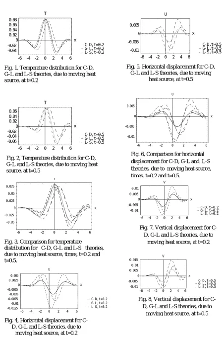
The values of real part oftemperature field and displacement components u(x,t)and v(x,t) are evaluated on the plane y = 1
for the problem of moving heat source and moving load. In Fig.1, three curves, predicted by the three theories, C-D, G-L and L-S for temperature distribution due to moving heat source at dimensionless time,
t
=
0
.
2
, are shown. The graph in Fig. 2, is drawn to see the variation in temperature at time5
.
0
=
t
whereas the comparison fortemperature variation, at time
t
=
0
.
2
and5
.
0
=
t
due to moving heat source is shown in Fig. 3. The horizontal displacement for C-D, G-L and L-S theories respectively due to moving heat source at dimensionless time2
.
0
=
t
andt
=
0
.
5
is shown in Fig. 4-5 and comparison of three theories is given in Fig.6. The graph in Fig. 7-8, is drawn to see vertical displacement at dimensionless timet
=
0
.
2
[image:6.595.72.282.71.579.2]-6 -4 -2 0 2 4 6 -0.04
-0.02 0 0.02 0.04 0.06 0.08
x T
L-S,t=0.2 G-L,t=0.2 C-D,t=0.2
-6 -4 -2 0 2 4 6 -0.06
-0.04 -0.02 0 0.02 0.04 0.06
x T
L-S,t=0.5 G-L,t=0.5 C-D,t=0.5
-6 -4 -2 0 2 4 6 -0.05
-0.025 0 0.025
0.05 0.075
x T
-6 -4 -2 0 2 4 6
-0.0125 -0.01 -0.0075
-0.005 -0.0025 0 0.0025
0.005
x U
L-S,t=0.2 G-L,t=0.2 C-D,t=0.2
-6 -4 -2 0 2 4 6 -0.01
-0.005 0 0.005
x U
L-S,t=0.5 G-L,t=0.5 C-D,t=0.5
-6 -4 -2 0 2 4 6
-0.01 -0.005 0 0.005
x U
-6 -4 -2 0 2 4 6
-0.01 -0.005 0 0.005
0.01
x V
L-S,t=0.2 G-L,t=0.2 C-D,t=0.2
-6 -4 -2 0 2 4 6 -0.01
-0.005 0 0.005
0.01 0.015
x V
L-S,t=0.5 G-L,t=0.5 C-D,t=0.5
[image:7.595.64.517.52.759.2]Fig. 1, Temperature distribution for C-D, G-L and L-S theories, due to moving heat source, at t=0.2
Fig. 2, Temperature distribution for C-D, G-L and L-S theories, due to moving heat source, at t=0.5
Fig. 3, Comparison for temperature
distribution for C-D, G-L and L-S theories, due to moving heat source, times, t=0.2 and t=0.5.
Fig. 4, Horizontal displacement for C-D, G-L and L-S theories, due to
[image:7.595.319.514.78.171.2]moving heat source, at t=0.2
Fig. 5, Horizontal displacement for C-D, G-L and L-S theories, due to moving
[image:7.595.80.275.79.171.2]heat source, at t=0.5
Fig. 6, Comparison for horizontal displacement for C-D, G-L and L-S theories, due to moving heat source, times, t=0.2 and t=0.5.
Fig. 7, Vertical displacement for C-D, G-L and L-S theories, due to
moving heat source, at t=0.2
Fig. 8, Vertical displacement for C-D, G-L and L-S theories, due to
[image:7.595.79.272.259.356.2]-6 -4 -2 0 2 4 6 -0.01
-0.005 0 0.005
0.01 0.015
x V
-6 -4 -2 0 2 4 6
-0.15 -0.1 -0.05 0 0.05
0.1 0.15
x T
L-S,t=0.2 G-L,t=0.2 C-D,t=0.2
-6 -4 -2 0 2 4 6
-0.1 -0.05 0 0.05
0.1 0.15
0.2
x T
L-S,t=0.5 G-L,t=0.5 C-D,t=0.5
-6 -4 -2 0 2 4 6
-0.15 -0.1 -0.05 0 0.05 0.1 0.15 0.2
x T
-6 -4 -2 0 2 4 6
-0.0075 -0.005 -0.0025 0 0.0025
0.005 0.0075
x U
L-S,t=0.2 G-L,t=0.2 C-D,t=0.2
-6 -4 -2 0 2 4 6
-0.01 -0.0075 -0.005 -0.0025 0 0.0025
0.005
x U
L-S,t=0.5 G-L,t=0.5 C-D,t=0.5
-6 -4 -2 0 2 4 6
-0.01 -0.0075 -0.005 -0.0025 0 0.0025
0.005 0.0075
x U
-6 -4 -2 0 2 4 6
-0.02 0 0.02 0.04
x V
[image:8.595.64.536.68.703.2]L-S,t=0.2 G-L,t=0.2 C-D,t=0.2
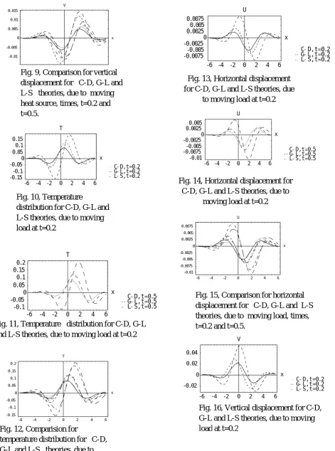
Fig. 12, Comparision for
temperature distribution for C-D, G-L and L-S theories, due to moving heat source, times, t=0.2
Fig. 13, Horizontal displacement for C-D, G-L and L-S theories, due
to moving load at t=0.2
Fig. 14, Horizontal displacement for C-D, G-L and L-S theories, due to
moving load at t=0.2
Fig. 15, Comparison for horizontal displacement for C-D, G-L and L-S theories, due to moving load, times, t=0.2 and t=0.5.
Fig. 16, Vertical displacement for C-D, G-L and L-S theories, due to moving load at t=0.2
Fig. 9, Comparison for vertical displacement for C-D, G-L and L-S theories, due to moving heat source, times, t=0.2 and t=0.5.
Fig. 11, Temperature distribution for C-D, G-L and L-S theories, due to moving load at t=0.2
Fig. 10, Temperature
[image:8.595.67.223.567.698.2]-6 -4 -2 0 2 4 6 -0.04
-0.02 0 0.02 0.04
x V
L-S,t=0.5 G-L,t=0.5 C-D,t=0.5
-6 -4 -2 0 2 4 6
-0.04 -0.02 0 0.02 0.04
x V
References
Acknowledgement: we are thankful to Prof. S.K. Tomar, Panjab University Chandigarh, India for the valuable suggestions during the preparation of this work .
References
[1] Lord, H. W., and Shulman, Y., 1967, .A generalized dynamical theory of thermoelasticity, J. Mech. Phys. Solids,Vol 15, pp. 299-309.
[2] Green, A. E., and Lindsay K. A., 1972, Thermoelasticity,.Journal of Elasticity, Vol.2, pp.1-7.
[3] Paria, G., 1967, Magnetoelasticity and Magnetothermoelasticity,. Adv.Appl.Mech, 10, pp. 73.
[4] Nayfeh, A. H., and Naser, S. N., 1972, .Electro Magnetothermoelastic plane waves in solids with thermal rexalation,.J. Appl. Mech. 113, pp.108-113.
[5] Chain, C. T., and Moon, F. C., 1981, Magnetically induced cylindrical stress waves in a thermoelastic conductor, Int. J. Solids Structures, 17, pp.1021-1035.
[6]Chaudhary,S.K.,1984,Electromagnetothermoela stic plane waves in rotating media with thermal rexalation,Int. J. Engng. Sci, 22, pp. 519-530.
[7] Sherief, H and Ezzat, M. A., 1996, A thermal shock problem in magneto thermoelasticity with thermal relaxation, Int .J. Solids Stuctures,33, pp. 4449-4459.
[9] Ezzat, M. A.,1997, State space approach to generalized magnetothermoelasticity with two relaxation times in a medium of perfect cond -uctivity,.Int. J. Engng. Sci., 35, pp.741-752. [10] Sherief, H., and Ezzat,M. A.,1998, A problem
in generalized magneto-thermoelasticity for an infinitely long annular cylinder, J. Engng. Math.34, pp. 387-402.
[11] Ezzat, M. A., Othman, M. I., and El-Karamany, A. S., 2001, Electromagneto-thermoelastic plane waves with thermal relaxation in a medium of perfect conductivity,.J. Thermal Stresses, 24, 411-432. [12] Ezzat, M. A., and El-Karamany, A. S., 2003,
Magnetothermoelasticity with two relaxation times in conducting medium with variable electrical and thermal conductivity, Appl. Math. Comp.,142, pp. 449-467.
[13] Massalas, C., and Dalmangas, A., 1983, .Coupled magnetothermoelastic problem in elastic half space,. Internat. J. Engrg. Sci. 21 (no. 2), pp.171-178.
[14] Chand D., Sharma J.N. and Sud S.P., 1990, Transient generalized magneto-thermoelastic waves in a rotating half-space,. International J.Engrg. Sci. 28 (no. 6),pp. 547.556.
[15] Roychoudhuri S.K. and Chatterjee (Roy) G., 1990, . A coupled magnetothermoelastic problem in a perfectly conducting elastic half-space with thermal relaxation,.Int. J. Math. Sci. 13 (no. 3), pp. 567.578.
[16] Roychoudhuri S.K., and Banerjee S., 1996, Magneto-thermo-elastic waves induced by a thermal shock in a infnitely conducting elastic half space, Int. J. Math. Math. Sci. 19 (no. 1), pp.131-143.
[17] Ezzat, M. A., 1997, .Generation of generalized magneto thermoelastic waves by thermal shock in a perfectly conducting half space,. J. Thermal stresses, 20, pp. 617-633.
[18] Othman, M. I. A., 2004, .Relaxation effects on thermal shock problems in an elastic half-space of generalized magneto- thermoelasticity,.J. of Mechanics and Mechanical Engineering, 7, pp.165-178.
[19] Roychoudri S.K.and Bandyoppadhya N.,2005 Magneto-thermoelastic waves in perfectly conducting elastic half space in thermoelasticty-III, Int. J. of Mathematics and Mathematical Sciences, Vol. 20, pp.3303-3318.
[20] Othman, M. I. A. and Song Y., 2007, Reflection of plane waves from an elastic solid half space and hydrostatic initial stress without energy dissipation, Int. J. of Solids and Structures, Vol.44, issue 17, pp.5651-5864. Fig. 17, Vertical displacement for
C-D, G-L and L-S theories, due to moving load, at t=0.5