B´ezier Curve for Trajectory Guidance

B´ezier Curve for Trajectory Guidance

Ji-wung Choi

, Gabriel Hugh Elkaim

Abstract—In this paper we present two path planning algorithms based on B´ezier curves for autonomous vehicles with waypoints and corridor constraints. B´ezier curves have useful properties for the path generation problem. The paper describes how the algorithms apply these properties to gen-erate the reference trajectory for vehicles to satisfy the path constraints. Both algorithms join cubic B´ezier curve segments smoothly to generate the path. Additionally, we discuss the constrained optimization problem that optimizes the resulting path for user-defined cost function. The simulation shows the generation of successful routes for autonomous vehicles using these algorithms as well as control results for a simple kine-matic vehicle. Extensions of these algorithms towards navigat-ing through an unstructured environment with limited sensor range are discussed.

Keywords: B´ezier, Path Planning, Optimization, Autonomous Vehicle, Feedback Control.

1. Introduction

Exploiting the versatility of autonomous vehicles for aca-demic, industrial, and military applications will have a pro-found effect on future applications. Current research on control systems for autonomous vehicles demonstrates that trajectory generation is hardly a “solved” problem. For ve-hicle viability, it is imperative to be able to generate safe paths in real time.

Many path planning techniques for autonomous vehi-cles have been discussed in the literature. Cornell Uni-versity Team for 2005 DARPA Grand Challenge [8] used a path planner based on B´ezier curves of degree3in a sens-ing/action feedback loop to generate smooth paths that are consistent with vehicle dynamics. Skrjanc [7] proposed a new cooperative collision avoidance method for multiple robots with constraints and known start and goal veloci-ties based on B´ezier curves of degree 5. In this method, four control points out of five are placed such that desired positions and velocities of the start and the goal point are satisfied. The fifth point is obtained by minimizing penalty functions. Lizarraga [5] used B´ezier curves for generating

∗_{Ph.D. Student, Autonomous Systems Lab, Computer Engineering}

De-partment, University of California, Santa Cruz, 95064, Tel: 831-428-2146, Email: jwchoi@soe.ucsc.edu

†_{Assistant Professor, Autonomous Systems Lab, Computer}

Engineer-ing Department, University of California, Santa Cruz, 95064, Tel: 831-459-3054, Email: elkaim@soe.ucsc.edu

spatially deconflicted paths for multiple UAVs.

Connors and Elkaim [1] previously presented a method for developing feasible paths through complicated environ-ments using a kernel function based on cubic splines. This method iteratively refines the path to compute a feasible path and thus find a collision free path in real time through an unstructured environment. This method, when imple-mented in a receding horizon fashion, becomes the basis for high level control. This previous method, however, re-sult in an incomplete path planning algorithm to satisfy the computational requirements in a complicated environment. A new approach has been developed based on using B´ezier curves as the seed function for the path planning algorithm as an alternative to cubic splines. The resulting path is ma-nipulated by the control points of the bounding polygon. Though the optimization function for collision avoidance is non-linear, it can be solved quickly and efficiently. The results of the new algorithm demonstrate the generation of higher performance, more efficient, and successful routes for autonomous vehicles. Feedback control is used to track the planned path. The new algorithm is validated using sim-ulations, and demonstrates a successful tracking result of a vehicle.

The paper is organized as follows: Section 2 begins by describing the definition of the B´ezier curve and its useful properties for path planning. Section 3 discusses the con-trol problem for autonomous vehicles, the vehicle dynam-ics, and vehicle control algorithms. Section 4 proposes four path planning methods of which two are based on B´ezier curves, and discusses the constrained optimization problem of these methods. In Section 5, simulation results of control problem for autonomous vehicles are given. Finally, Sec-tion 6 provides conclusions and future work.

2. B´ezier Curve

B´ezier Curves were invented in 1962 by the French engi-neer Pierre B´ezier for designing automobile bodies. Today B´ezier Curves are widely used in computer graphics and an-imation [6]. A B´ezier Curve of degreencan be represented as

P[t0,t1](t) =

n

X

i=0

Where Pi are control points such that P(t0) = P0 and

P(t1) =Pn,Bni(t)is a Bernstein polynomial given by

B_in(t) =

n i

(t1−t

t1−t0)

n−i₍t−t0 t1−t0)

i_{, i}

∈ {0,1, . . . , n}

B´ezier Curves have useful properties for path planning:

• They always passes throughP0andPn.

• They are always tangent to the lines connectingP0→

P1andPn→Pn−1atP0andPnrespectively.

• They always lie within the convex hull consisting of their control points.

2.1. The de Casteljau Algorithm

The de Casteljau Algorithm is named after the French math-ematician Paul de Casteljau, who developed the algorithm in 1959. The de Casteljau algorithm describes a recursive process to subdivide a B´ezier curveP[t0,t2](t)into two

seg-mentsP[t0,t1](t)andP[t1,t2](t)[6]. Let{P

0

0, P10, . . . , Pn0}

denote the control points ofP[t0,t2](t). The control points

ofP[t0,t1](t)andP[t1,t2](t)can be computed by

P_ij=(1−τ)P_ij−1+τ P_ij₊₁−1,

j∈ {1, . . . , n}, i∈ {0, . . . , n−j} (1)

whereτ = t1−t0

t2−t0. Then,{P

0

0, P01, . . . , P0n}are the control

points ofP[t0,t1]and{P

n

0, P1n−1, . . . , Pn0}are the control

points ofP[t1,t2].

Remark 1. A B´ezier curveP[t0,t2] always passes through

the pointP(t1) =P0ncomputed by applying the de

Castel-jau algorithm to subdivide itself intoP[t0,t1] andP[t1,t2].

Also, it is always tangent toP₀n−1P₁n−1atP(t1).

The path planning method introduced in the Section 4.3.2 is motivated by this property.

2.2. Derivatives

The derivatives of a B´ezier curve, referred to as the hodo-graph, can be determined by its control points [6]. For a B´ezier curveP[t0,t1](t) =

Pn

i=0B

n

i(t)Pi, the first

deriva-tive can be represented as:

˙

P[t0,t1](t) =

n−1 X

i=0

B_in−1(t)Di (2)

WhereDi, control points ofP˙[t0,t1](t)is

Di =

n

t1−t0(Pi+1−P i)

The higher order derivative of a B´ezier curve can be ob-tained by using the relationship of Equation (2).

2.3. Curvature

The curvature of andegree B´ezier curveP[t0,t1]at its

end-point is given by [6]

κ(t0) =n−1

n

h0

|P0−P1|2 (3)

κ(t1) = n−1

n

h1

|Pn−1−Pn|2

(4)

Whereh0is the distance fromP2to the line segmentP0P1,

h1is the distance fromPN−2to the line segmentPn−1Pn.

3. Problem Statement

Consider the control problem of a ground vehicle with a mission defined by waypoints and corridor constraints in a two-dimensional free-space. Our goal is to develop and implement an algorithm for navigation that satisfies these constraints. Let us denote each waypoint Wi ∈ R2 for

i ∈ {1,2, . . . , N}, where N ∈ Ris the total number of

waypoints. Corridor width is denoted aswj,j-th widths of

each segment between two waypoints,j∈ {1, . . . , N−1}.

3.1. Dynamic Model of Vehicle Motion

This section describes a dynamic model for motion of a vehicle that is used in the simulation in Section 5. For the dynamics of the vehicle, the state and the control vec-tor are denoted q(t) = (xc(t), yc(t), ψ(t))T andu(t) =

(v(t), ω(t))T _{respectively. Where (x}

c, yc)represents the

position of the center of gravity of the vehicle. The vehi-cle yaw angle ψis defined to the angle from theX axis.

vis the longitudinal velocity of the vehicle at the center of gravity.ω= ˙ψis the yaw angular velocity. It follows that

˙ q(t) =





cosψ(t) 0 sinψ(t) 0

0 1



u(t)

3.2. Controls

The vehicle uses feed forward path planning with feedback corrections as illustrated in Figure 1 [4]. A position and ori-entation error is computed every 50ms. The cross track errorycerr is defined by the shortest distance between the

reference trajectory and the position of the center of gravity of the vehicle(xc, yc). A pointcis computed with the

cur-rent longitudinal velocity and heading of the vehicle from the current position. cis projected onto the reference tra-jectory at pointpsuch that cpis normal to the tangent at

p. The cross track erroryerris defined by the distance

be-tweencandp. The steering controlωuses PID controller with respect to cross track erroryerr.

˙

ω=kpyerr+kd

dyerr

dt +ki Z

yerrdt

Figure 1: The position error of the vehicle is measured from a pointc, projected in front of the vehicle, and unto the ideal curve to pointp.

4. Path Planning Algorithm

In this section, four path planning methods are proposed. To describe the methods, we consider the course with way-pointsW = {Wi}, i ∈ {1, . . . , N} and corridor width

wk = 8, k ∈ {1, . . . , N −1} for N = 4 as

illus-trated in Figure 2. The location of waypoints are given by two-dimensional world coordinates (X, Y) in meter

scale: W1 = (10,5), W2 = (55,20), W3 = (47,65),

W4= (70,50).

To describe the algorithms, let us denotelj as the

bisec-tor of_∠Wj−1WjWj+1 for j ∈ {2, . . . , N −1} and mj

as the normal line tolj at the intersect of the planned path

andlj. The course is divided into segments Gk bylk+1. Gk indicates the permitted area for vehicles under corridor

constraintwk, fromWktoWk+1.

4.1. Path Planning Based on Center Lines

The simplest path planning method is to follow a series of center lines that connect neighboring waypoints, plotted as a black line in Figure 2. Although this method has advan-tages of simplicity and optimality in terms of the shortest path, the sharp turns at waypoints are not feasible for ve-hicles in practice. It will result in a position error varying as a function of the longitudinal velocity and the maximum steer angle. Section 5 details the simulation and Figure 6(a) shows the result of this path.

4.2. Path Planning Using Circular Arcs for

Turns

To reduce position error at segment transitions with sharp turns, another path planning method is proposed with cir-cular arc. Under the assumption that the slip angle of the vehicle is zero in lateral motion, the ideal shape of a path

Figure 2: The course with four waypoints. Gray area is the per-mitted area for vehicles under a corridor constraint.

with a turn is a circular arc as it has constant radius of cur-vature. Figure 3 shows the potential trajectories aroundW2. They consist of a circular arc and its tangents. It is interest-ing to note the followinterest-ing property from the geometry.

Remark 2. The tangent of the trajectory on the bisectorlj

is normal tolj.

This property will be used as a constraint of the path planning methods introduced in the Section 4.3.1 and 4.3.2.

Figure 3:An enlarged path based on circular arc for a turn atW2.

4.3. Path Planning Based on B´ezier Curves

In this section, two methods of path planning based on B´ezier curves are proposed. Both methods are motivated by Remark 2 and are developed to preserve it.

point with different desired velocities. The least degree of the B´ezier curve that can satisfy this requirement is three (See properties of B´ezier curves in Section 2). Both meth-ods use a set of cubic B´ezier curves.

The cubic B´ezier curves used for the path planning are denoted as P[ti−1,ti](t) =

P3

k=0B 3

k(t)Pk,i for i ∈

{1, . . . , M} where M is the total number of the B´ezier curves. The planned pathP(t)for t ∈ [t0, tM] is

repre-sented as

P(t) ={P[ti−1,ti](t)}, i∈ {1, . . . , M}

4.3.1 Path Planning Placing B´ezier Curves within Seg-ments

In this path planning method, the cubic B´ezier curves

P[ti−1,ti](t) =

P3

k=0B 3

k(t)Pk,i for i ∈ {1, . . . , N −1}

are used within each segmentGias shown in Figure 4. The

planned pathP(t)are designed such that it begins fromW1

with the heading of−−−−→W1W2and ends toWN with the

head-ing of−−−−−−−→WN−1WN. Furthermore, the corridor constraint and

Remark 2 are satisfied.

Figure 4: The planned path based on cubic B´ezier curves used within segments whenTi =Wi. The B´ezier curves are plotted

with different colors: blue, black, and red.

The control points ofP[ti−1,ti](t), Pk,i are determined to maintain these conditions. The beginning point of

P[t0,t1](t), P0,1 isW1. The end point ofP[tN−2,tN−1](t),

P3,N−1isWN. Other beginning/end points denoted asTj

are chosen on the bisectorslj forj ∈ {2, . . . , N −1}and

bounded within the corridor. Then it is assigned toP3,j−1

andP0,j. {P0,i, P1,i, P2,i, P3,i}always lie within the area

ofGiso that the resulting B´ezier curve satisfies the corridor

constraint by the convex hull property. Also,{P1,i, P2,i}

are chosen such that the derivatives ofP[tj−2,tj−1](t) and

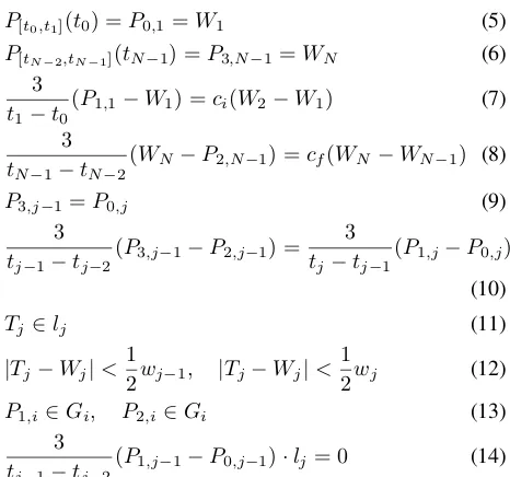
P[tj−1,tj](t)atTjare continuous and are normal tolj. These can be formulated as the following constraints:

P[t0,t1](t0) =P0,1=W1 (5)

P[tN−2,tN−1](tN−1) =P3,N−1=WN (6)

3

t1−t0(P1,1−W1) =ci(W2−W1) (7)

3

tN−1−tN−2

(WN−P2,N−1) =cf(WN−WN−1) (8)

P3,j−1=P0,j (9)

3

tj−1−tj−2

(P3,j−1−P2,j−1) =

3

tj−tj−1

(P1,j−P0,j)

(10)

Tj ∈lj (11)

|Tj−Wj|<

1

2wj−1, |Tj−Wj|< 1

2wj (12)

P1,i∈Gi, P2,i∈Gi (13)

3

tj−1−tj−2

(P1,j−1−P0,j−1)·lj = 0 (14)

Whereci ∈R,cf ∈Rand velocity constraints (7), (8),

and (14) are represented by applying (2). [ti−1, ti]are

as-sumed to be given. ThenP={P1,i, P2,i}andT={Tj}

are computed by minimizing the constrained optimization problem:

min

P,TJ =

N−1 X

i=1

Ji (15)

subject to (7), (8), (10), (11), (12), (13), and (14).

Where Ji is the cost function of P[ti−1,ti](t) which is defined in Section 5. As the result, the planned trajectory passes through {W1, T2, . . . , TN−2, WN−1} with Remark

2 preserved.

4.3.2 Path Planning Placing Mid-points of B´ezier Curves on Bisectors of Turns

In the section 4.3.1, a B´ezier curve is used within each seg-ment. Another path planning method places the mid-points of the B´ezier curves on the bisectorslj,j ∈ {2, . . . , N−1}

using the de Casteljau algorithm. In this method, cubic B´ezier curves P[ti−1,ti](t) =

P3

k=0B 3

k(t)Pk,i0 for i ∈

{1, . . . ,2N−3}are used.

The local area of the course aroundWj can be seen as

symmetric with respect tolj. Thus the cubic B´ezier curves

P[ti0 −1,ti0](t),i0 ∈ {2,4, . . . ,2N−4}used for this area will

also be symmetric with respect toli0_/2+1. In other words,

P₀0_,i0 andP₃0_,i0are symmetric with respect toli0_/2+1. So are

P0

1,i0 andP₂0_,i0. After applying the de Casteljau algorithm withτ = 0.5to the curve, the mid-pointP3

0,i0is onli0_/2+1. Then B´ezier curvesP[t_i00 −1,ti00](t)fori

00_{∈ {1,3, . . . ,2N−}

3} are used for the rest part of the path. The constraints imposed on the planned path are as follows:

Figure 5:The path based on cubic B´ezier curves placed such that their mid-point lies on the bisectors.

P₀0_,1=W1 (16)

P30,2N−3=WN (17)

3

t1−t0

(P₁0_,1−W1) =ci(W2−W1) (18)

3

t2N−4−t2N−3

(WN −P20,2N−3) =cf(WN −WN−1)

(19)

P₃0_,i=P₀0_,i+1 (20) 3

ti−ti−1

(P₃0_,i−P₂0_,i) = 3

ti+1−ti

(P₁0_,i+1−P₀0_,i+1)

(21)

(P₀0_,i0+P₃0_,i0)/2 ∈li0_/2+1

(P0

1,i0+P₂0_,i0)/2 ∈li0_/2+1

(22)

P₃0_,i0 ∈Gi0_/2 (23)

P₀0_,i0 ∈Gi0_/2

1 2P

0

0,i0+1₂P₁0_,i0 ∈Gi0_/2

1 4P

0

0,i0+1₂P₁0_,i0+1₄P₂0_,i0 ∈Gi0_/2

 



(24)

|1 8P

0

0,i0+3₈P₁0_,i0+3₈P₂0_,i0+1₈P₃0_,i0| <1₂wi0_/2 |1

8P 0

0,i0+3₈P₁0_,i0+3₈P₂0_,i0+1₈P₃0_,i0| <1₂wi0_/2+1

(25)

P₁0_,i00∈G_(i00_+1)/2, P₂0_,i00∈G_(i00_+1)/2 (26)

Where ci ∈ R, cf ∈ R, and boundary constraints

(24) and (25) are represented by applying (1). [ti−1, ti]

are assumed to be given. Then P = {P0

0,i0, P₁0_,i0} and

Q= {P0

1,i00, P₂0_,i00}are computed by minimizing the con-strained optimization problem:

min

P,QJ = 2N−3

X

i=1

Ji (27)

subject to (18), (19), (21), (22), (24), (25), and (26). Remarkable feature of this method is the fact that it poses desirable position and velocity of the mid-point of a B´ezier curve as well as those of the beginning and the end points. Furthermore, the convex hull property is tested for{P₀0_,i0, P₀1_,i0, P₀2_,i0, P₀3_,i0}of the divided curves in-stead of{P0

0,i0, P₁0_,i0, P₂0_,i0, P₃0_,i0}. Since the curve and the course is locally symmetrical, we do not need to check {P3

0,i0, P₁2_,i0, P₂1_,i0, P₃0_,i0}. As the result, it comes up with more tight condition for curves against the corridor con-straint than checking{P0

0,i0, P₁0_,i0, P₂0_,i0, P₃0_,i0}by perform-ing the same number of tests.

5. Simulation Results

(a) Line (b) Arc

(c) B´ezier1 (d) B´ezier2

Figure 6: Tracking simulation results (blue) over the planned paths (black).

Simulation performed in this paper uses the course as shown in Figure 2. Initial position and heading are assumed to fit to the first waypoint and the direction to the second waypoint respectively. The constant longitudinal velocity

v(t) = 10m/sis used. The magnitude of ω is bounded within|ω|max= 2.618rad/s. The PID gains are given by:

kp= 2,kd= 1, andki= 0.1.

(a) The steering controlω. (b) The cross track errorycerr.

Figure 7:The steering controlωand the cross track errorycerr.

the planned path byLineis shown in Figure 6(a). Although the vehicle tracks the straight parts of the planned path ac-curately, it overshoots in turns resulting in a large position error due to maximum steer angle limitation. Decreasing speed as the vehicle approaches to the turning area can re-duce the position error. However, in this simulation, the longitudinal velocityv was kept constant which magnifies the tracking errors with this method of path planning.

Figure 6(b) shows the tracking result of Arc. Where uniform radius R = 5 is used. It satisfies the condition

ofR ≥ v

|ω|max = 3.8197for vehicles to converge to the planned circular arc path.

Figure 6(c) is the tracking result over the path planned by B´ezier1. This path obtained by solving Equation (15) with

Ji=

Z ti

ti−1

h

( ˙P[ti−1,ti](t))

2_{+ ( ¨P}

[ti−1,ti](t))

2i_dt

Whereti =i. JipenalizesP˙ andP¨ to give smoothness to

each B´ezier curve.

Figure 6(d) is the tracking result over the path planned byB´ezier2. This path obtained by solving Equation (27) with

Ji=

Z ti

ti−1

h

( ˙P[ti−1,ti](t))

2_{+ ( ¨P}

[ti−1,ti](t))

2i_dt,

i∈ {1,3, . . . ,2N−3}

(28)

Ji=

Z ti

ti−1

h

( ˙P[ti−1,ti](t))

2_{+ ( ¨P}

[ti−1,ti](t))

2i_dt+ 20 κ(ti)

,

i∈ {2,4, . . . ,2N−4}

(29)

Note that two differentJiare used. B´ezier curves used in

turns are additionally penalized inversely to the curvature at their endpoints in Equation (29). This leads to a resulting path with smooth turns.

6. Summary and Conclusions

This paper presents two path planning algorithms based on B´ezier curves for autonomous vehicles with waypoints and

corridor constraints. B´ezier curves provide an efficient way to generate the optimized path and satisfy the constraints at the same time. The simulation results also show that the trajectory of the vehicle converges to the planned path suc-cessfully.

These path planning algorithms will be implemented on the Overbot [4], the autonomous ground vehicle at Au-tonomous Systems Lab in UCSC.

In this work, proposed algorithms only generate nominal path. We will extend and expand our work in receding hori-zon obstacle avoidance for an autonomous ground vehicle. Enabling autonomous vehicles to detect unknown obstacles and safely avoid them is essential to future operations. Ad-ditionally, receding horizon control methods will be applied to generate real-time B´ezier-based optimal trajectories.

References

[1] J. Connors, G. Elkaim, “Analysis of a Spline Based, Obstacle Avoiding Path Planning Algorithm,”IEEE Vehicle Technol-ogy Conference, IEEE VTC 2007,Dublin, Ireland, Apr. 22-25, 2007

[2] J. Connors, G. Elkaim, “Experimental Results for Spline Based Obstacle Avoidance of an Off-Road Ground Vehicle,” ION Global Navigation Satellite Systems Conference, ION GNSS 2007,Fort Worth, TX, Sept. 25-28, 2007

[3] J. Connors, G. Elkaim, “Manipulating B-Spline Based Paths for Obstacle Avoidance in Autonomous Ground Vehicles,” ION National Technical Meeting, ION NTM 2007,San Diego, CA, Jan. 22-24, 2007

[4] G. Elkaim, J. Connors, and J. Nagel, “The Overbot: An off-road autonomous ground vehicle testbed,”ION Global Nav-igation Satellite Systems Conference (ION-GNSS 2006), 1, Sept. p.22-24, 2006.

[5] M. Lizarraga, G. Elkaim, “Spatially Deconflicted Path Gener-ation for Multiple UAVs in a Bounded Airspace,”ION/IEEE Position, Location, and Navigation Symposium, ION/IEEE PLANS 2008,Monterey, CA, May 5-8, 2008

[6] T. W. Sederber, “Computer aided geometric design,”CAGD Course Notes,Brigham Young University, Provo, UT, 84602, April 2007.

[7] I. Skrjanc, G. Klancar “Cooperative Collision Avoidance be-tween Multiple Robots Based on Bzier Curves,”Information Technology Interfaces, 2007 (ITI 2007),p.451-456, June 25-28, 2007.

[8] The 2005 DARPA Grand Challenge,vol. 36/2007, p.363-405, Springer Berlin / Heidelberg, 2007.