Regularized Minimum Error Rate Training

Regularized Minimum Error Rate Training

Michel Galley

Microsoft Research [email protected]

Chris Quirk

Microsoft Research [email protected]

Colin Cherry

National Research Council [email protected]

Kristina Toutanova

Microsoft Research [email protected]

Abstract

Minimum Error Rate Training (MERT) re-mains one of the preferred methods for tun-ing linear parameters in machine translation systems, yet it faces significant issues. First, MERT is an unregularized learner and is there-fore prone to overfitting. Second, it is com-monly used on a noisy, non-convex loss func-tion that becomes more difficult to optimize as the number of parameters increases. To ad-dress these issues, we study the addition of a regularization term to the MERT objective function. Since standard regularizers such as `2are inapplicable to MERT due to the scale

invariance of its objective function, we turn to two regularizers—`0and a modification of`2—

and present methods for efficiently integrating them during search. To improve search in large parameter spaces, we also present a new direc-tion finding algorithm that uses the gradient of expected BLEU to orient MERT’s exact line searches. Experiments with up to 3600 features show that these extensions of MERT yield re-sults comparable to PRO, a learner often used with large feature sets.

1 Introduction

Minimum Error Rate Training emerged a decade ago (Och, 2003) as a superior training method for small numbers of linear model parameters of machine translation systems, improving over prior work using maximum likelihood criteria (Och and Ney, 2002). This technique quickly rose to prominence, becom-ing standard in many research and commercial MT systems. Variants operating over lattices (Macherey et al., 2008) or hypergraphs (Kumar et al., 2009) were subsequently developed, with the benefit of reducing the approximation error from n-best lists.

The primary advantages of MERT are twofold. It directly optimizes the evaluation metric under consid-eration (e.g., BLEU) instead of some surrogate loss.

Secondly, it offers a globally optimal line search. Un-fortunately, there are several potential difficulties in scaling MERT to larger numbers of features, due to its non-convex loss function and its lack of reg-ularization. These challenges have prompted some researchers to move away from MERT, in favor of lin-early decomposable approximations of the evaluation metric (Chiang et al., 2009; Hopkins and May, 2011; Cherry and Foster, 2012), which correspond to easier optimization problems and which naturally incorpo-rate regularization. In particular, recent work (Chiang et al., 2009) has shown that adding thousands or tens of thousands of features can improve MT quality when weights are optimized using a margin-based approximation. On simulated datasets, Hopkins and May (2011) found that conventional MERT strug-gles to find reasonable parameter vectors, where a smooth loss function based on Pairwise Ranking Op-timization (PRO) performs much better; on real data, this PRO method appears at least as good as MERT on small feature sets, and also scales better as the number of features increases.

In this paper, we seek to preserve the advantages of MERT while addressing its shortcomings in terms of regularization and search. The idea of adding a regularization term to the MERT objective function can be perplexing at first, because the most common regularizers, such as`1and`2, are not directly appli-cable to MERT. Indeed, these regularizers arescale sensitive, while the MERT objective function is not: scaling the weight vector neither changes the predic-tions of the linear model nor affects the error count. Hence, MERT can hedge any regularization penalty by maximally scaling down linear model weights.

The first contribution of this paper is to analyze var-ious forms of regularization that are not susceptible to this scaling problem. We analyze and experiment with`0, a form of regularization that isscale

insen-sitive. We also present new parameterizations of`2

regularization, where we apply`2regularization to scale-senstive linear transforms of the original linear model. In addition, we introduce efficient methods of incorporating regularization in Och (2003)’s exact line searches. For all of these regularizers, our meth-ods let us find the true optimum of the regularized objective function along the line.

Finally, we address the issue of searching in a high-dimensional space by using the gradient of ex-pected BLEU (Smith and Eisner, 2006) to find better search directions for our line searches. This direction finder addresses one of the serious concerns raised by Hopkins and May (2011): MERT widely failed to reach the optimum of a synthetic linear objective function. In replicating Hopkins and May’s experi-ments, we confirm that existing search algorithms for MERT—including coordinate ascent, Powell’s algo-rithm (Powell, 1964), and random direction sets (Cer et al., 2008)—perform poorly in this experimental condition. However, when using our gradient-based direction finder, MERT has no problem finding the true optimum even in a 1000-dimensional space.

Our results suggest that the combination of a reg-ularized objective function and a gradient-informed line search algorithm enables MERT to scale well with a large number of features. Experiments with up to 3600 features show that these extensions of MERT yield results comparable to PRO (Hopkins and May, 2011), a parameter tuning method known to be effective with large feature sets.

2 Unregularized MERT

Prior to introducing regularized MERT, we briefly review standard unregularized MERT (Och, 2003). We use fS₁ = {f1. . .fS}to denote theSinput

sen-tences of a given tuning set. For each sentencef_s, let C_s={e_s,1. . .e_s,M}denote the list ofM-best can-didate translations. Each input and output sentence pair(f_s,e_s,m)is weighted using a linear model that applies model parameters w = (w₁. . . w_D) ∈ _RD

to D feature functions h₁(f,e,∼). . . h_D(f,e,∼), where ∼ is the hidden state associated with the derivation from f to e, such as phrase segmenta-tion and alignment. Furthermore, let hs,m ∈ RD

denote the feature vector representing the translation pair(fs,es,m).

In MERT, the goal is to minimize a loss function

E(r,e)that scores translation hypotheses against a

set of reference translationsrS₁ ={r1. . .rS}. This

yields the following optimization problem:

ˆ

w= arg min

w

S

X

s=1

E(rs,ˆe(fs;w))

=

arg min

w

S

X

s=1

M X

m=1

E(rs,es,m)δ(es,m,ˆe(fs;w))

(1) where

ˆe(f_s;w) = arg max

m∈{1...M}

w|h_s,m (2)

While the error surface of Equation 1 is only an approximation of the true error surface of the MT decoder, the quality of this approximation depends on the size of the hypothesis space represented by the

M-best list. Therefore, the hypothesis list is grown iteratively: decoding with an initial parameter vector seeds the M-best lists; next, parameter estimation andM-best list gathering alternate until the cumula-tiveM-best list no longer grows, or until changes of wbetween two decoding runs are deemed too small. To increase the size of the hypothesis space, subse-quent work (Macherey et al., 2008) instead operated on lattices, but this paper focuses onM-best lists.

A crucial observation is that the unsmoothed error count represented in Equation 1 is a piecewise con-stant function. This enabled Och (2003) to devise a line search algorithm guaranteed to find the optimum point along the line. To extend the search from one to multiple dimensions, MERT applies a sequence of line optimizations along some fixed or variable set of search directions{dt}until some convergence

criteria are met. Considering a given pointwtand

a given directiond_tat iterationt, finding the most probable translation hypothesis in the set of candi-dates translationsC_s={e_s,1. . .e_s,M}corresponds to solving the following optimization problem:

ˆe(fs;γ) = arg max m∈{1...M}

(wt+γ·dt)|hs,m

(3)

defined by the pointsγfs

1 <· · ·< γ fs

M at which an

in-crease inγcauses a change of optimum in Equation 3. Error counts for the whole corpus are simply the sums of sentence-level piecewise constant functions aggre-gated over all sentences of the corpus.1The optimalγ

is finally computed by enumerating all piecewise con-stant intervals of the corpus-level error function, and by selecting the one that has the lowest error count (or, correspondingly, highest BLEU score). Assum-ing the optimum is found in the interval[γ_k−1, γk],

we defineγ_opt = (γ_k−1+γk)/2and change the

pa-rameters using the updatewt+1=wt+γopt·dt.

Finally, this method is turned into a global D -dimensional search using algorithms that repeat-edly use the aforementioned exact line search algo-rithm. Och (2003) first advocated the use of Powell’s method (Powell, 1964; Press et al., 2007). Pharaoh (Koehn, 2004) and subsequently Moses (Koehn et al., 2007) instead use coordinate ascent, and more recent work often uses random search directions (Cer et al., 2008; Macherey et al., 2008). In Section 4, we will present a novel direction finder for maximum-BLEU optimization, which uses the gradient of expected BLEU to find directions where the BLEU score is most likely to increase.

3 Regularization for MERT

Because MERT is prone to overfitting when a large number of parameters must be optimized, we study the addition of a regularization term to the objective function. One conventional approach is to regularize the objective function with a penalty based on the

Euclidean norm||w||2 =

q P

iw2i, also known as`2

regularization. In the case of MERT, this yields the following objective function:2

ˆ

w= arg min

w

S

X

s=1

E(r_s,ˆe(f_s;w)) +||w|| 2 2 2σ2

(4)

1

This assumes that the sufficient statistics of the metric under consideration are additively decomposable by sentence, which is the case with most popular evaluation metrics such as BLEU (Papineni et al., 2001).

2

The`2regularizer is often used in conjunction with log-likelihood objectives. The regularization term of Equation 4 could similarly be added to the log of an objective—e.g.,

log(BLEU)instead of BLEU—but we found that the distinc-tion doesn’t have much of an impact in practice.

-0.20 0.2 0.4 0.6 0.81 1.2 1.4

-0.4 -0.3 -0.2 -0.1 0 0.1 0.2 0.3 0.4 MERT

Max at 0.225

× ×

-0.20 0.2 0.4 0.6 0.81 1.2 1.4

-0.4 -0.3 -0.2 -0.1 0 0.1 0.2 0.3 0.4 MERT−`2

Max at -0.018

×

× −`2

-0.20 0.2 0.4 0.6 0.81 1.2 1.4

-0.4 -0.3 -0.2 -0.1 0 0.1 0.2 0.3 0.4 γ, the step size in the current direction

MERT−`0

Max at 0

×

×

`0

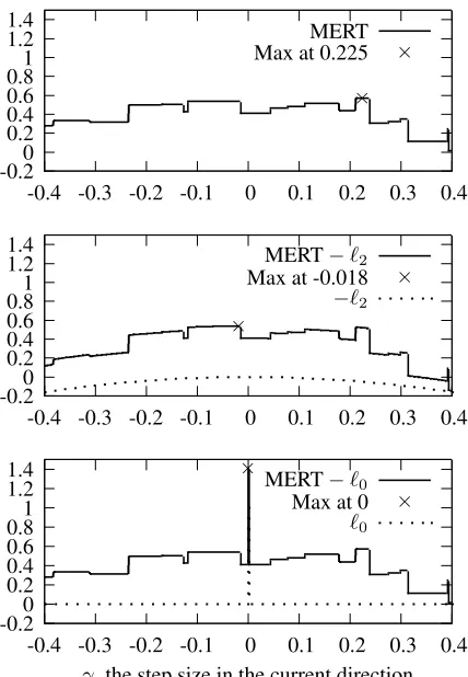
Figure 1: Example MERT values along one coordi-nate, first unregularized. When regularized with`2, the

piecewise constant function becomes piecewise quadratic. When using`0, the function remains piecewise constant

with a point discontinuity at 0.

where the regularization term1/2σ2is a free param-eter that controls the strength of the regularization penalty. Similar regularizers have also been used in conjunction with other norms, such as`<sub>1</sub>and`₀

norms. The`₁ norm, defined as ||w||₁ = P i|wi|,

applies a constant force toward zero, preferring vec-tors with fewer non-zero components;`₀, defined as

||w||0 =|{i|wi 6= 0}|, simply counts the number of

non-zero components of the weight vector, encoding a preference for sparse vectors.

reg-ularization terms, the function respectively becomes piecewise quadratic, piecewise linear, or piecewise constant with a potential impulse jump for each dis-tinct choice of regularizer. Figure 1 demonstrates this effect graphically.

As discussed in (McAllester and Keshet, 2011), the problem with optimizing Equation 4 directly is that the output of the underlying linear classifier, and therefore the error count, are not sensitive to the scale ofw. Moreover,`<sub>2</sub>regularization (as well as`₁ reg-ularization) is scale sensitive, which means any op-timizer of this function can drive the regularization term down to zero by scaling down w. As special treatments for`2, we evaluate three linear transforms of the weight vector, where the vectorwof the regu-larization term||w||2

2/2σ2is replaced with either:

1. an affine transform:w−w0

2. a vector with only(D−1)free parameters, e.g., (1, w0₂,· · ·, w_D0 )

3. an`₁renormalization:w/||w||₁

In (1), regularization is biased towardsw0, a weight vector previously optimized using a competitive yet much smaller feature set, such as core features of a phrase-based (Koehn et al., 2007) or hierarchical (Chiang, 2007) system. The requirement that this feature set be small is to prevent overfitting. Other-wise, any regularization toward an overfit parameter vectorw0 would defeat the purpose of introducing a regularization term in the first place.3 In (2), the transformation is motivated by the observation that the D-parameter linear model of Equation 2 only needs(D−1) degrees of freedom. Fixing one of the components ofwto any non-zero constant and allowing the others to vary, the new linear model re-tains the same modeling power, but the(D−1)free parameters are no longer scale invariant, i.e., scaling the(D−1)-dimensional vector now has an effect on linear model predictions. In (3), the weight vector is normalized as to have an`1-norm equal to 1. In contrast, the `0 norm is scale insensitive, thus not affected by this problem.

3.1 Exact line search with regularization

Optimizing with a regularized error surface requires a change in the line search algorithm presented in

3

(Gimpel and Smith, 2012, footnote 6) briefly mentions the use of such a regularizer with its ramp loss objective function.

Section 2, but the other aspects of MERT remain the same, and we can still use global search algorithms such as coordinate ascent, Powell, and random di-rections exactly the same way as with unregularized MERT. Line search with a regularization term is still as efficient as in (Och, 2003), and it is still guar-anteed to find the optimum of the (now regularized) objective function along the line. Considering again a given pointwtand a given directiondtat line search

iterationt, finding the optimumγ_optcorresponds to findingγ that minimizes:

S X

s=1

E(rs,ˆe(fs;γ)) +

||wt+γ·dt||22

2σ2 (5)

Since regularization does not affect the points at which ˆe(f_s;γ) changes its optimum, the points

γfs

1 <· · ·< γ fs

M of intersection in the upper

enve-lope remain the same, so the points of discontinuity in the error surface remain the same. The difference now is that the error count on each segment[γi−1, γi]

is no longer constant. This means we need to adjust the final step of line search, which consists of enu-merating all[γi−1, γi], and keeping the optimum of

Equation 5 for each segment.ˆe(fs;γ)remains

con-stant within the segment, so we only need to consider the expression ||wt+γ ·dt||22 to select a segment point. The optimum is either at the left edge, the right edge, or in the middle if the vertex of the parabola happens to lie within that segment.4 _{We compute} this optimum by finding the valueγ for which the derivative of the regularization term is zero. There is an easy closed-form solution:

d dγ

||wt+γ·dt||22 2σ2

= 0

d dγ

X

i

(w2_t,i+ 2·γ·w_t,i·d_t,i+γ2·d2_t,i)

= 0

X

i

(2·w_t,i·d_t,i+ 2·γ·d2_t,i) = 0

γ =− X i

w_t,i·d_t,i X i

d2_t,i

=−wt|dt

d_t|d_t

This closed-form solution is computed in time pro-portional to D, which doesn’t slow down the

com-4

When the optimum is either at the left edgeγi−1or right edgeγiof a segment, we select a point at a small relative distance

within the segment (.999γi−1+.001γi, in the former case) to

putation of Equation 5 for each segment (the con-struction of each segment of the upper envelope is proportional toDanyway).

We also use `<sub>0</sub> regularization. While minimiza-tion of the`₀-norm is known to be NP-hard in gen-eral (Hyder and Mahata, 2009), this optimization is relatively trivial in the case of a line search. Indeed, for a given segment, the value in Equation 5 is con-stant everywhere except where we intersect any of the coordinate hyperplanes, i.e., where one of the coordinates is zero. Thus, our method consists of evaluating Equation 5 at the intersection points be-tween the line and coordinate hyperplanes, returning the optimal point within the given segment. For any segment that doesn’t cross any of these hyperplanes, we evaluate the objective function at any point of the segment (since the value is constant across the entire segment).

4 Direction finding

4.1 A Gradient-based direction finder

Perhaps the greatest obstacle in scaling MERT to many dimensions is finding good search direc-tions. In problems of lower dimensions, iterating through all the coordinates is computationally feasi-ble, though not guaranteed to find a global maximum even in the case of a perfect line search. As the number of dimensions increases by orders of mag-nitude, this coordinate direction approach becomes less and less tractable, and the quality of the search also suffers (Hopkins and May, 2011).

Optimization has traditionally relied on finding the direction of steepest ascent: the gradient. Unfortu-nately, the objective function optimized by MERT is piecewise constant; while it may admit a subgradi-ent, this direction is generally not very informative. Instead we may consider a smoothed variation of the original approximation. While some variants have been considered (Och, 2003; Flanigan et al., 2013), we use an expected BLEU approximation, assum-ing hypotheses are drawn from a log-linear distri-bution according to their parameter values (Smith and Eisner, 2006). That is, we assume the proba-bility of a translation candidatee_s,mis proportional to(exp (w|h_s,m))µ, whereware the parameters be-ing optimized,hs,mis the vector of the features for

es,m, andµis a scaling parameter. Asµapproaches

infinity, the distribution places all its weight on the highest scoring candidate.

The log of the BLEU score may be written as:

min

1−R C,0

+ 1

N N X

n=1

(logmn−logcn)

whereRis the sum of reference lengths across the corpus,Cis the sum of candidate lengths,mnis the

number of matched n-grams (potentially clipped), andcnis the number ofn-grams in all candidates.

Given a distribution over candidates, we can use the expected value of the log of the BLEU score. This is a smooth approximation to the BLEU score, which asymptotically approaches the true BLEU score as the scaling parameterµapproaches infinity. While this expectation is difficult to compute exactly, we can compute approximations thereof using Taylor se-ries. Although prior work demonstrates that a second-order Taylor approximation is feasible to compute (Smith and Eisner, 2006), we find that a first-order approximation is faster and very close to the second-order approximation.5The first order Taylor approxi-mation is as follows:

min

1− R

E[C],0

+1

N N X

n=1

(logE[mn]−logE[cn])

whereEis the expectation operator using the

proba-bility distributionP(h;w, µ). First we note that the gradient_∂w∂

iP(h;w, µ)is

P(h;w, µ) hi− X

h0

h0_iP(h0;w, µ)

!

Using the chain rule, the gradient of the first order approximation to BLEU is as follows:

1

N N X

n=1

1

E[mn] X

h

mn(h)

∂P(h;w, µ)

∂wi

− 1

E[cn] X

h cn(h)

∂P(h;w, µ)

∂w_i

+

(

0 ifE[C]> R

R

E[C]2

P

hc1(h)∂P(_∂wh;w_i,µ) otherwise

5

In the case of`2-regularized MERT, the final gradi-ent also includes the partial derivative of the regular-ization penalty of Equation 4, which iswi/σ2for a

given componentiof the gradient. We do not update the gradient in the case of`0 regularization since the

`₀-norm is not differentiable.

4.2 Search

Our search strategy consists of looking at the direc-tions of steepest increase of expected BLEU, which is similar to that of Smith and Eisner (2006), but with the difference that we do so in the context of MERT. We think this difference provides two benefits. First, while the smooth approximation of BLEU reduces the likelihood of remaining trapped in a local opti-mum, we avoid approximation error by retaining the original objective function. Second, the benefit of exact line searches in MERT is that there is no need to be concerned about step size, since step size in MERT line searches is guaranteed to be optimal with respect to the direction under consideration.

Finally, our gradient-based search algorithm oper-ates as follows. Considering the current pointwt, we

compute the gradientgtof the first order Taylor

ap-proximation at that point, using the current scaling pa-rameterµ. (We initialize the search withµ= 0.01.) We find the optimum along the linew_t+γ·g_t. When-ever any given line search yields no improvement larger than a small tolerance threshold, we multiply

µby two and perform a new line search. The increase of this parameterµcorresponds to a cooling schedule (Smith and Eisner, 2006), which progressively sharp-ens the objective function to get a better estimate of BLEU as the search converges to an optimum. We repeatedly perform new line searches untilµexceeds 1000. The inability to improve the current optimum with a sharp approximation (µ >1000) doesn’t mean line searches would fail with smaller values, so we find it helpful to repeat the above procedure until a full pass of updates ofµfrom 0.01 to 1000 yields no improvement.

4.3 Computational complexity

Computing the gradient increases the computational cost of MERT, though not its asymptotic complexity. The cost of a single exhaustive line search is

O(SM(D+ logM+ logS))

whereS is the number of sentences, each with M

possible translations, andDis the number of features. For each sentence, we first identify the model score as a linear function of the step size, requiring two dot products for an overall cost ofO(SM D).6 Next we construct the upper envelope for each sentence: first the equations are sorted in increasing order of slope, and then they are merged in linear time to form an envelope, with an overall cost ofO(SMlogM). A linear pass through the envelope converts these into piecewise constant (or linear, or quadratic) repre-sentations of the (regularized) loss function. Finally the per-sentence envelopes are merged into a global representation of the loss along that direction. Our implementation successively merges adjacent pairs of piecewise smooth loss function representations until a single list remains. TheselogSpasses lead to a merging runtime ofO(SMlogS).

The time required to compute a gradient is pro-portional toO(SM D). For each sentence, we first gather the probability and its gradient, then use this to compute expected n-gram counts and matches as well as those gradients in timeO(M D). A constant num-ber of arithmetic operations suffice to compute the final expected loss value and its gradient. Therefore, computing the gradient does not increase the algo-rithmic complexity when compared to conventional approaches using coordinate ascent and random di-rections. Likewise the runtime of a single iteration is competitive with PRO, given that gradient finding is generally the most expensive part of convex opti-mization. Of course, it is difficult to compare overall runtime of convex optimization with that of MERT, as we know of no way to bound the number of gradi-ent evaluations required for convergence with MERT. Therefore, we resort to empirical comparison later in the paper, and find that the two methods appear to have comparable runtime.

6

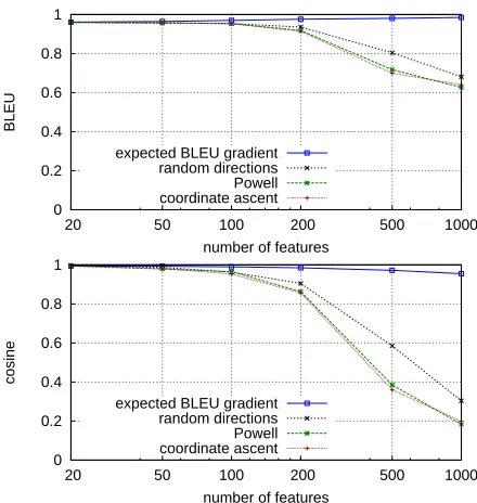
Language pair Train Tune Dev Test

GBM

Chinese-English 0.99M 1,797 1,000 1,082 (mt02+03) (mt05) Finnish-English 2.20M 11,935 2,001 4,855

SparseHRM

Chinese-English 3.51M 1,894 1,664 1,357 (mt05) (mt06) (mt08) Arabic-English 1.49M 1,663 1,360 1,313 (mt06) (mt08) (mt09)

Table 1: Datasets for the two experimental conditions.

5 Experimental Design

Following Hopkins and May (2011), our experimen-tal setup utilizes both real and synthetic data. The motivation for using synthetic data is that it is a way of gauging the quality of optimization methods, since the data is constructed knowing the global optimum. Hopkins and May also note that the use of an ob-jective function that is linear in some gold weight vector makes the search much simpler than in a real translation setting, and they suggest that a learner that performs poorly in such a simple scenario has little hope of succeeding in a more complex one.

The setup of our synthetic data experiment is al-most the same as that performed by Hopkins and May (2011). We generate feature vectors of dimen-sionality ranging from 10 to 1000. These features are generated by drawing random numbers uniformly in the interval[0,500]. This synthetic dataset consists of S=1000 source “sentences”, and M=500 “trans-lation” hypotheses for each sentence. A pseudo “BLEU” score is then computed for each

hypothe-sis, by computing the dot product between a prede-fined gold weight vectorw∗and each feature vector hs,m. By this linear construction,w∗is guaranteed

to be a global optimum.7 The pseudo-BLEU score is normalized for eachM-best list, so that the transla-tion with highest model score according tow∗ has a BLEU score of 1, and so that the translation with lowest model score for the sentence gets a BLEU of zero. This normalization has no impact on search, but makes results more interpretable.

For our translation experiments, we use multi-stack phrase-based decoding (Koehn et al., 2007). We report results for two feature sets: non-linear features induced using Gradient Boosting Machines (Toutanova and Ahn, 2013) and sparse lexicalized

7

The objective function remains piecewise constant, and the plateau containingw∗maps to the optimalvalueof the function.

reordering features (Cherry, 2013). We exploit these feature sets (GBMandSparseHRM, respectively) in two distinct experimental conditions, which we de-tail in the two next paragraphs. Both GBM and

SparseHRM augment baseline features similar to Moses’: relative frequency and lexicalized phrase translation scores for both translation directions; one or two language model features, depending on the language pair; distortion penalty; word and phrase count; six lexicalized reordering features. For both experimental conditions, phrase tables have maxi-mum phrase length of 7 words on either side. In reference to Table 1, we used the training set (Train) for extracting phrase tables and language models; the

Tuneset for optimization with MERT or PRO; the

Devset for selecting hyperparameters of PRO and regularized MERT; and theTestset for reporting fi-nal results. In each experimental condition, we first trained weights for the base feature sets, and then decoded theTune,Dev, andTestdatasets, generating 500-best lists for each set. All results report rerank-ing performance on these lists with different feature sets and optimization methods, based on lower-cased BLEU (Papineni et al., 2001).

TheGBMfeature set (Toutanova and Ahn, 2013) consists of about 230 features automatically induced using decision tree weak learners, which derive fea-tures using various word-level, phrase-level, and mor-phological attributes. For Chinese-English, the train-ing corpus consists of approximately one million sen-tence pairs from the FBIS and Hong Kong portions of the LDC data for the NIST MT evaluation and the

TuneandTestsets are from NIST competitions. A 4-gram language model was trained on the Xinhua portion of the English Gigaword corpus and on the target side of the bitext. For Finnish-English we used a dataset from a technical domain of software man-uals. For this language pair we used two language models: one very large model trained on billions of words, and another language model trained from the target side of the parallel training set.

0 0.2 0.4 0.6 0.8 1

50 100 500 1000

20 200

BLEU

number of features expected BLEU gradient

random directions Powell coordinate ascent

0 0.2 0.4 0.6 0.8 1

50 100 500 1000

20 200

cosine

number of features expected BLEU gradient

random directions Powell coordinate ascent

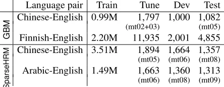
Figure 2: Change in BLEU score and cosine similarity to the gold weight vectorw∗_{as the number of features}

increases, using the noisysynthetic experiments. The gradient-based direction finding method is barely affected by the noise. The increase of the number of dimensions en-ables our direction finder to find a slightly better optimum, which moved away fromw∗due to noise.

language models were trained on the target side of the parallel training data for both Arabic and Chinese. The Chinese systems development set is taken from the NIST mt05 evaluation set, augmented with some material reserved from our NIST training corpora in order to better cover newsgroup and weblog domains.

6 Results

We conducted experiments with the synthetic data scenario described in the previous section, as well as with noise added to the data (Hopkins and May, 2011). The purpose of adding noise is to make the optimization task more realistic. Specifically, af-ter computing all pseudo-BLEU scores, we added noise to each feature vectorh_s,m by drawing from a zero-mean Gaussian with standard deviation 200. Our results with both noiseless and noisy data yield the same conclusion as Hopkins and May: standard MERT struggles with many dimensions, and fails to recoverw∗. However, our experiments with the gradient direction finder of Section 4 are much more positive. This direction finder not only recoversw∗

40 50 60 70 80 90 100

1 10 100 1000

BLEU

line search iteration expected BLEU gradient (noisy) expected BLEU gradient coordinate ascent (noisy) coordinate ascent

Figure 3: Comparison of rate of convergence between coordinate ascent and our expected BLEU direction finder (D= 500).Noisyrefers to the noisy experimental setting.

(cosine>0.999) even with 1000 dimensions, but its effectiveness is also visible with noisy data, as seen in Figure 2. The decrease of its cosine is relatively small compared to other search algorithms, and this decrease is not necessarily a sign of search errors since the addition of noise causes the true optimum to be different fromw∗. Finally, Figure 3 shows our rate of convergence compared to coordinate ascent.

Our experimental results with the GBM feature set data are shown in Table 2. Each table is di-vided into three sections corresponding respectively to MERT (Och, 2003) with Koehn-style coordinate ascent (Koehn, 2004), PRO, and our optimizer featur-ing both regularization and the gradient-based direc-tion finder. All variants of MERT are initialized with a single starting point, which is either uniform weight orw₀. Instead of providing MERT with additional random starting points as in Moses, we use random walks as in (Moore and Quirk, 2008) to attempt to move out of local optima.8 Since PRO and our opti-mizer have hyperparameters, we use a held-out set (Dev) for adjusting them. For PRO, we adjust three parameters: a regularization penalty for `2, the pa-rameterαin the add-αsmoothed sentence-level ver-sion of BLEU (Lin and Och, 2004), and a parameter for scaling the corpus-level length of the references. The latter scaling parameter is discussed in (He and

8

Chinese-English Finnish-English Method Starting pt. # feat. Tune Dev Test # feat. Tune Dev Test

MERT uniform 14 33.2 19.9 32.9 15 53.0 52.6 54.8

MERT uniform 224 33.0 19.2 32.1 232 53.2 51.7 53.8

MERT w0 224 34.1 20.1 33.0 232 53.9 52.5 54.7

PRO w0 224 33.4 20.1 33.3 232 53.3 52.9 55.3

`2MERT (v1:||w−w0||) w0 224 33.2 20.3 33.5 232 53.2 52.7 55.2

`2MERT (v2:D−1dimensions) w0 224 33.0 20.4 33.2 232 52.9 52.6 55.0

`2MERT (v3:`1-renormalized) w0 224 33.1 20.0 33.3 232 53.1 52.5 55.1

`0MERT w0 224 33.4 20.3 33.2 232 53.2 52.6 55.1

Table 2: BLEU scores forGBMfeatures. Model parameters were optimized on theTuneset. For PRO and regularized MERT, we optimized with different hyperparameters (regularization weight, etc.), and retained for each experimental condition the model that worked best onDev. The table shows the performance of these retained models.

51.2 51.4 51.6 51.8 52 52.2 52.4 52.6

1e-05 0.0001 0.001 0.01 0.1 1 10

BLEU

regularization weight expected BLEU gradient

coordinate ascent

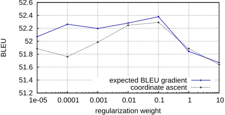
Figure 4: BLEU score on the Finnish Dev set (GBM) with different values for the1/2σ2_{regularization weight.}

To enable comparable results, the other hyperparameter (length) is kept fixed.

Deng, 2012; Nakov et al., 2012) and addresses the problem that systems tuned with PRO tend to pro-duce sentences that are too short. On the other hand, regularized MERT only requires one hyperparameter to tune: a regularization penalty for`2 or`0. How-ever, since PRO optimizes translation length on the

Devdataset and MERT does so using theTuneset, a comparison of the two systems would yield a discrep-ancy in length that would be undesirable. Therefore, we add another hyperparameter to regularized MERT to tune length in the same manner using theDevset. Table 2 offers several findings. First, unregular-ized MERT can achieve competitive results with a small set of highly engineered features, but adding a large set of more than 200 features causes MERT to perform poorly, particularly on the test set. However, unregularized MERT can recover much of this drop of performance if it is given a good sparse initializer w0. Regularized MERT (v1) provides an increase in the order of 0.5 BLEU on the test set compared to

the best results with unregularized MERT. Regular-ized MERT is competitive with PRO, even though the number of features is relatively large. Using the same

GBMexperimental setting, Figure 4 compares regu-larized MERT using the gradient direction finder and coordinate ascent. At the best regularization setting, the two algorithms are comparable in terms of BLEU (though coordinate ascent is slower due to its lack of a good direction finder), but our method seems more robust with suboptimal regularization parameters.

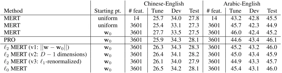
Our results with theSparseHRMfeature set data are shown in Table 3. As with theGBMfeature set, we find again that the version of`₂ MERT regular-ized towards ||w−w₀|| is competitive with PRO, even though we train MERT with a large set of 3601 features.9 _{One remaining question is whether MERT} remains practical with large feature sets. As noted in the complexity analysis of Section 4.3, MERT has a dependence on the number of features that is comparable to PRO, i.e., it is linear in both cases. Practically, we find that optimization time is com-parable between the two systems. In the case of Chinese-English for theGBMfeature set, one run of the PRO optimizer took 26 minutes on average, while regularized MERT with the gradient direction finder took 37 minutes on average, taking into account the time to computew₀. In the case of Chinese-English for theSparseHRMfeature set, average optimization times for PRO and our method were 3.10 hours and 3.84 hours on average, respectively.

9

Chinese-English Arabic-English Method Starting pt. # feat. Tune Dev Test # feat. Tune Dev Test

MERT uniform 14 25.7 34.0 27.8 14 43.2 42.8 45.5

MERT uniform 3601 25.4 33.1 27.3 3601 45.7 42.3 44.9

MERT w0 3601 27.7 33.5 27.5 3601 46.0 42.4 45.2

PRO w0 3601 25.9 34.3 28.1 3601 44.6 43.4 46.1

`2MERT (v1:||w−w0||) w0 3601 26.3 34.3 28.3 3601 45.2 43.2 46.0

`2MERT (v2:D−1dimensions) w0 3601 26.4 34.1 28.2 3601 45.0 43.4 45.9

`2MERT (v3:`1-renormalized) w0 3601 26.1 34.0 27.9 3601 44.9 43.3 45.7

`0MERT w0 3601 26.5 34.2 28.1 3601 45.4 43.1 46.0

Table 3: BLEU scores forSparseHRMfeatures. Notes in Table 2 also apply here.

Finally, as shown in Table 2, we see that MERT ex-periments that rely on a good initial starting pointw₀ generally perform better than when starting from a uniform vector. While having to compute w₀ in the first place is a bit of a disadvantage compared to standard MERT, the need for good initializer is hardly surprising in the context of non-convex op-timization. Other non-convex problems in machine learning, such as deep neural networks (DNN) and word alignment models, commonly require such ini-tializers in order to obtain decent performance. In the case of DNN, extensive research is devoted to the problem of finding good initializers.10 In the case of word alignment, it is common practice to initialize search in non-convex optimization problems—such as IBM Model 3 and 4 (Brown et al., 1993)—with solutions of simpler models—such as IBM Model 1.

7 Related work

MERT and its extensions have been the target of ex-tensive research (Och, 2003; Macherey et al., 2008; Cer et al., 2008; Moore and Quirk, 2008; Kumar et al., 2009; Galley and Quirk, 2011). More recent work has focused on replacing MERT with a linearly de-composable approximations of the evaluation metric (Smith and Eisner, 2006; Liang et al., 2006; Watan-abe et al., 2007; Chiang et al., 2008; Hopkins and May, 2011; Rosti et al., 2011; Gimpel and Smith, 2012; Cherry and Foster, 2012), which generally involve a surrogate loss function incorporating a reg-ularization term such as the`2-norm. While we are not aware of any previous work adding a penalty on

10

For example, (Larochelle et al., 2009) presents a pre-trained DNN that outperforms a shallow network, but the performance of the DNN becomes much worse relative to the shallow network once pre-training is turned off.

the weights in the context of MERT, (Cer et al., 2008) achieves a related effect. Cer et al.’s goal is to achieve a more regular or smooth objective function, while ours is to obtain a more regular set of parameters. The two approaches may be complementary.

More recently, new research has explored direction finding using a smooth surrogate loss function (Flani-gan et al., 2013). Although this method is successful in helping MERT find better directions, it also exac-erbates the tendency of MERT to overfit.11 As an indirect way of controlling overfitting on the tuning set, their line searches are performed over directions estimated over a separate dataset.

8 Conclusion

In this paper, we have shown that MERT can scale to a much larger number of features than previously thought, thanks to regularization and a direction finder that directs the search towards the greatest increase of expected BLEU score. While our best results are comparable to PRO and not significantly better, we think that this paper provides a deeper un-derstanding of why standard MERT can fail when handling an increasingly larger number of features. Furthermore, this paper complements the analysis by Hopkins and May (2011) of the differences be-tween MERT and optimization with a surrogate loss function.

Acknowledgments

We thank the anonymous reviewers for their helpful comments and suggestions.

11

References

Peter F. Brown, Vincent J. Della Pietra, Stephen A. Della Pietra, and Robert L. Mercer. 1993. The mathematics of statistical machine translation: parameter estimation.

Comput. Linguist., 19(2):263–311.

Daniel Cer, Dan Jurafsky, and Christopher D. Manning. 2008. Regularization and search for minimum error rate training. InProceedings of the Third Workshop on Statistical Machine Translation, pages 26–34. Colin Cherry and George Foster. 2012. Batch tuning

strategies for statistical machine translation. In Pro-ceedings of the 2012 Conference of the North American Chapter of the Association for Computational Linguis-tics: Human Language Technologies, pages 427–436. Colin Cherry. 2013. Improved reordering for

phrase-based translation using sparse features. InProceedings of the 2013 Conference of the North American Chap-ter of the Association for Computational Linguistics: Human Language Technologies, pages 22–31.

David Chiang, Yuval Marton, and Philip Resnik. 2008. Online large-margin training of syntactic and structural translation features. InProceedings of the 2008 Con-ference on Empirical Methods in Natural Language Processing, pages 224–233.

David Chiang, Kevin Knight, and Wei Wang. 2009. 11,001 new features for statistical machine translation. InProceedings of Human Language Technologies: The 2009 Annual Conference of the North American Chap-ter of the Association for Computational Linguistics, pages 218–226.

David Chiang. 2007. Hierarchical phrase-based transla-tion. Computational Linguistics, 33(2):201–228. Jeffrey Flanigan, Chris Dyer, and Jaime Carbonell. 2013.

Large-scale discriminative training for statistical ma-chine translation using held-out line search. In Pro-ceedings of the 2013 Conference of the North American Chapter of the Association for Computational Linguis-tics: Human Language Technologies, pages 248–258. Michel Galley and Chris Quirk. 2011. Optimal search

for minimum error rate training. In Proceedings of the 2011 Conference on Empirical Methods in Natural Language Processing, pages 38–49.

Kevin Gimpel and Noah A. Smith. 2012. Structured ramp loss minimization for machine translation. In Proceed-ings of the 2012 Conference of the North American Chapter of the Association for Computational Linguis-tics: Human Language Technologies, pages 221–231. Xiaodong He and Li Deng. 2012. Maximum expected

BLEU training of phrase and lexicon translation mod-els. In Proceedings of the 50th Annual Meeting of the Association for Computational Linguistics: Long Papers - Volume 1, pages 292–301.

Mark Hopkins and Jonathan May. 2011. Tuning as rank-ing. InProceedings of the 2011 Conference on Empir-ical Methods in Natural Language Processing, pages 1352–1362.

M. Hyder and K. Mahata. 2009. An approximate L0 norm minimization algorithm for compressed sens-ing. In Acoustics, Speech and Signal Processing, 2009. ICASSP 2009. IEEE International Conference on, pages 3365–3368.

Philipp Koehn, Hieu Hoang, Alexandra Birch Mayne, Christopher Callison-Burch, Marcello Federico, Nicola Bertoldi, Brooke Cowan, Wade Shen, Christine Moran, Richard Zens, Chris Dyer, Ondrej Bojar, Alexandra Constantin, and Evan Herbst. 2007. Moses: Open source toolkit for statistical machine translation. In

Proc. of ACL, Demonstration Session.

Philipp Koehn. 2004. Pharaoh: a beam search decoder for phrase-based statistical machine translation models. InProc. of AMTA, pages 115–124.

Shankar Kumar, Wolfgang Macherey, Chris Dyer, and Franz Och. 2009. Efficient minimum error rate train-ing and minimum bayes-risk decodtrain-ing for translation hypergraphs and lattices. InProceedings of the Joint Conference of the 47th Annual Meeting of the ACL and the 4th International Joint Conference on Natural Language Processing of the AFNLP, pages 163–171. Hugo Larochelle, Yoshua Bengio, J´erˆome Louradour, and

Pascal Lamblin. 2009. Exploring strategies for training deep neural networks.J. Mach. Learn. Res., 10:1–40. P. Liang, A. Bouchard-Cˆot´e, D. Klein, and B. Taskar.

2006. An end-to-end discriminative approach to ma-chine translation. InInternational Conference on Com-putational Linguistics and Association for Computa-tional Linguistics (COLING/ACL).

Chin-Yew Lin and Franz Josef Och. 2004. ORANGE: a method for evaluating automatic evaluation metrics for machine translation. InProceedings of the 20th international conference on Computational Linguistics, Stroudsburg, PA, USA.

Wolfgang Macherey, Franz Och, Ignacio Thayer, and Jakob Uszkoreit. 2008. Lattice-based minimum error rate training for statistical machine translation. In Pro-ceedings of the 2008 Conference on Empirical Methods in Natural Language Processing, pages 725–734. David McAllester and Joseph Keshet. 2011.

Generaliza-tion bounds and consistency for latent structural probit and ramp loss. InAdvances in Neural Information Processing Systems 24, pages 2205–2212.

Preslav Nakov, Francisco Guzman, and Stephan Vogel. 2012. Optimizing for sentence-level BLEU+1 yields short translations. InProceedings of COLING 2012, pages 1979–1994.

Franz Josef Och and Hermann Ney. 2002. Discriminative training and maximum entropy models for statistical machine translation. InProceedings of 40th Annual Meeting of the Association for Computational Linguis-tics, pages 295–302.

Franz Josef Och. 2003. Minimum error rate training in statistical machine translation. InProceedings of the 41st Annual Meeting of the Association for Computa-tional Linguistics, pages 160–167.

Kishore Papineni, Salim Roukos, Todd Ward, and Wei-Jing Zhu. 2001. BLEU: a method for automatic evalu-ation of machine translevalu-ation. InProc. of ACL.

Kishore Papineni. 1999. Discriminative training via linear programming. InProceedings IEEE International Con-ference on Acoustics, Speech, and Signal Processing (ICASSP), volume 2, pages 561–564, Vol. 2.

M.J.D. Powell. 1964. An efficient method for finding the minimum of a function of several variables without calculating derivatives. Comput. J., 7(2):155–162. William H. Press, Saul A. Teukolsky, William T.

Vetter-ling, and Brian P. Flannery. 2007. Numerical Recipes: The Art of Scientific Computing. Cambridge University Press, 3rd edition.

Antti-Veikko Rosti, Bing Zhang, Spyros Matsoukas, and Richard Schwartz. 2011. Expected BLEU training for graphs: BBN system description for WMT11 sys-tem combination task. In Proceedings of the Sixth Workshop on Statistical Machine Translation, pages 159–165.

David A. Smith and Jason Eisner. 2006. Minimum risk annealing for training log-linear models. In Proceed-ings of the COLING/ACL 2006 Main Conference Poster Sessions, pages 787–794.