Random Manhattan Integer Indexing:
Incremental
L1
Normed Vector Space Construction
Behrang Q. Zadeh††Insight Centre
National University of Ireland, Galway Galway, Ireland
Siegfried Handschuh†‡
‡Dept. of Computer Science and Mathematics
University of Passau Bavaria, Germany
Abstract
Vector space models (VSMs) are math-ematically well-defined frameworks that have been widely used in the distributional approaches to semantics. In VSMs, high-dimensional vectors represent linguistic entities. In an application, the similar-ity of vectors—and thus the entities that they represent—is computed by a distance formula. The high dimensionality of vec-tors, however, is a barrier to the perfor-mance of methods that employ VSMs. Consequently, a dimensionality reduction technique is employed to alleviate this problem. This paper introduces a novel technique called Random Manhattan In-dexing (RMI) for the construction of `1
normed VSMs at reduced dimensionality. RMI combines the construction of a VSM and dimension reduction into an incre-mental and thus scalable two-step proce-dure. In order to attain its goal, RMI em-ploys the sparse Cauchy random projec-tions. We further introduce Random Man-hattan Integer Indexing (RMII): a compu-tationally enhanced version of RMI. As shown in the reported experiments, RMI and RMII can be used reliably to estimate the`1 distances between vectors in a vec-tor space of low dimensionality.
1 Introduction
Distributional semantics embraces a set of meth-ods that decipher the meaning of linguistic en-tities using their usages in large corpora (Lenci, 2008). In these methods, the distributional proper-ties of linguistic entiproper-ties in various contexts, which are collected from their observations in corpora, are compared to quantify their meaning. Vector spaces are intuitive, mathematically well-defined
frameworks to represent and process such infor-mation.1 In a vector space model (VSM), linguis-tic entities are represented by vectors and a dis-tance formula is employed to measure their distri-butional similarities (Turney and Pantel, 2010).
In a VSM, each element~siof the standard basis of the vector space (informally, each dimension of the VSM) represents a context element. Givenn
context elements, an entity whose meaning is be-ing analyzed is expressed by a vector~vas a linear combination of ~si and scalars αi ∈ R such that ~v=α1~s1+· · ·+αn~sn. The value ofαiis derived from the frequency of the occurrences of the entity that~v represents in/with the context element that
~si represents. As a result, the values assigned to the coordinates of a vector (i.e.αi) exhibit the
cor-relation of entities and context elements in ann -dimensional real vector spaceRn. Each vector can
be written as a1×nrow matrix, e.g.(α1,· · · , αn).
Therefore, a group ofmvectors in a vector space is often represented by a matrixMm×n.
Latent semantic analysis (LSA) is a famil-iar technique that employs a word-by-document
VSM (Deerwester et al., 1990).2 In this word-by-document model, the meaning of words (i.e. the linguistic entities) is described by their occur-rences in documents (i.e. the context elements). Given m words and n distinct documents, each word is represented by an n-dimensional vector
~vi= (αi1,· · · , αin), whereαij is a numeric value
that associates the word ~vi represents to the
doc-ument dj, for 1 < j < n. For instance, the value of αij may correspond to the frequency of
the word in the document. It is hypothesized that the relevance of words can be assessed by count-ing the documents in which they co-occur. There-fore, words with similar vectors are assumed to have the same meaning (Figure1).
1Amongst other representation frameworks.
2See Martin and Berry (2007) for an overview of the
mathematical foundation of LSA.
~s1↔d1 ~s2↔d2
~s3↔d3
~ v1 ~
v2
α12
α11
α13
α22
α21
α23
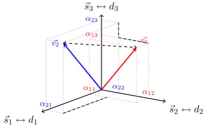
Figure 1: Illustration of a word-by-document
model consisting of 2 words and 3 documents. The words are represented in a3-dimensional vec-tor space, in which each ~si (each dimension) rep-resents each of the 3 documents in the model.
~v1 = (α11, α12, α13) and ~v2 = (α21, α22, α23)
represent the two words in the model. The dashed line shows the Euclidean distance between the two vectors that represent words, while the sum of dash-dotted lines is the Manhattan distance be-tween them.
In order to assess the similarity between vectors, a vector space V is endowed with a norm struc-ture. A norm k.k is a function that maps vectors from V to the set of non-negative real numbers, i.e.V 7→[0,∞). The pair of(V,k.k)is then called a normed space. In a normed space, the similar-ity between vectors is assessed by their distances. The distance between vectors is defined by a func-tion that satisfies certain axioms and assigns a real value to each pair of vectors, i.e.
dist:V ×V 7→R, d(~v,~t) =k~v−~uk. (1) The smaller the distance between two vectors, the more similar they are.
Euclidean space is the most familiar example of a normed space. It is a vector space that is en-dowed by the`2norm. In Euclidean space, the`2
norm—which is also called the Euclidean norm— of a vector~v= (v1,· · ·, vn)is defined as
k~vk2= v u u tXn
i=1 v2
i. (2)
Using the definition of distance given in Equa-tion 1and the`2 norm, the Euclidean distance is
measured as
dist2(~v, ~u) =k~v−~uk2 = v u u tXn
i=1
(vi−ui)2. (3)
In Figure1, the dashed line shows the Euclidean distance between the two vectors. In `2 normed
vector spaces, various similarity metrics are de-fined using different normalization of the Eu-clidean distance between vectors, e.g. the cosine similarity.
The similarity between vectors, however, can also be computed in`1 normed spaces.3 The `1 norm for~vis given by
k~vk1 = n X
i=1
|vi|, (4)
where|.|signifies the modulus. The distance in an
`1 normed vector space is often called the Man-hattanor thecity blockdistance. According to the definition given in Equation1, the Manhattan dis-tance between two vectors~vand~uis given by
dist1(~v, ~u) =k~v−~uk1 = n X
k=1
|vi−uj|. (5)
In Figure1, the collection of the dash-dotted lines is the`1distance between the two vectors. Similar
to the`2 spaces, various normalizations of the`1
distance4 define a family of`1 normed similarity metrics.
As the number of text units that are being mod-elled in a VSM increases, the number of context elements that are required to be utilized to capture their meaning escalates. This phenomenon is ex-plained using power-law distributions of text units in context elements (e.g. the familiar Zipfian dis-tribution of words). As a result, extremely high-dimensional vectors, which are also sparse—i.e. most of the elements of the vectors are zero— represent text units. The high dimensionality of the vectors results in setbacks, which are colloqui-ally known asthe curse of dimensionality. For in-stance, in a word-by-document model that consists of a large number of documents, a word appears only in a few documents, and the rest of the doc-uments are irrelevant to the meaning of the word. Few common documents between words results in sparsity of the vectors; and the presence of irrele-vant documents introduces noise.
Dimension reduction, which usually follows the construction of a VSM, alleviates the problems
3The definition of the norm is generalized to`
pspaces
withk~vkp = Pi|vi|p1/p, which is beyond the scope of
this paper.
[image:2.595.77.284.64.190.2]listed above by reducing the number of context el-ements that are employed for the construction of the VSM. In its simple form, dimensionality re-duction can be performed using a selection pro-cess: choose a subset of contexts and eliminate the rest using a heuristic. Alternatively, transfor-mationmethods can be employed. A transforma-tion method maps a vector spaceVnonto aVm of
lowered dimension, i.e. τ : Vn 7→ Vm, m n. The vector space at reduced dimension, i.e. Vm,
is often the best approximation of the originalVn
in asense. LSA employs a dimension reduction technique called truncated singular value decom-position (SVD). In a standard truncated SVD, the transformation guarantees the least distortion in the`2distances.5
Besides the problem of high computational complexity of SVD computation,6 which can be addressed by incremental techniques (see e.g. Brand (2006)), matrix factorization methods such as truncated SVD are data-sensitive: if the struc-ture of the data being analyzed changes, i.e. when either the linguistic entities or context elements are updated, e.g. some are removed or new ones are added, the transformation should be recom-puted and reapplied to the whole VSM to reflect the updates. In addition, a VSM at the original high dimension must be first constructed. Follow-ing the construction of the VSM, the dimension of the VSM is reduced in an independent process. Therefore, the VSM at reduced dimension is avail-able for processing only after the whole sequence of these processes. Construction of the VSM at its original dimension is computationally expen-sive and a delay in access to the VSM at reduced dimension is not desirable. Hence, the application of truncated SVD is not suitable in several appli-cations, particularly when dealing with frequently updated big text–data such as applications in the web context.
Random indexing (RI) is an alternative method that solves the problems stated above by combin-ing the construction of a vector space and the di-mensionality reduction process. RI, which is in-troduced in Kanerva et al. (2000), constructs a VSM directly at reduced dimension. Unlike meth-ods that first construct a VSM at its original high dimension and conduct a dimensionality reduction
5Please note that there are matrix factorization techniques
that guarantee the least distortion in the`1distances, see e.g. Kwak (2008).
6Matrix factorization techniques, in general.
afterwards, the RI method avoids the construction of the original high-dimensional VSM. Instead, it merges the vector space construction and the di-mensionality reduction process. RI, thus, signifi-cantly enhances the computational complexity of deriving a VSM from text. However, the appli-cation of the RI technique (likewise the standard truncated SVD in LSA) is limited to `2 normed
spaces, i.e. when similarities are assessed using a measure based on the`2distance. It can be verified
that using RI causes large distortions in the`1
dis-tances between vectors (Brinkman and Charikar, 2005). Hence, if the similarities are computed us-ing the `1 distance, then the RI technique is not
suitable for the VSM construction.
Depending on the distribution of vectors in a VSM, the performance of similarity measures based on the`1and the`2 norms varies from one
task to another. For instance, it is known that the `1 distance is more robust to the presence of outliers and non-Gaussian noise than the `2
dis-tance (e.g. see the problem description inKe and Kanade (2003)). Hence, the `1 distance can be more reliable than the`2 distance in certain appli-cations. For instance,Weeds et al. (2005) suggest that the `1 distance outperforms other similarity
metrics in a term classification task. In another experiment, Lee (1999) observed that the`1
dis-tance gives more desirable results than the Cosine and the`2measures.
In this paper, we introduce a novel method called Random Manhattan Indexing(RMI). RMI constructs a vector space model directly at re-duced dimension while it preserves the pairwise
`1 distances between vectors in the original high-dimensional VSM. We then introduced a compu-tationally enhanced version of RMI called Ran-dom Manhattan Integer Indexing (RMII). RMI and RMII, similar to RI, merge the construction of a VSM and dimension reduction into an incre-mental and thus efficient and scalable process.
In Section2, we explain and evaluate the RMI method. In Section 3, the RMII method is ex-plained. We compare the proposed method with RI in Section4. We conclude in Section5.
2 Random Manhattan Indexing
procedure: (a) the creation ofindex vectorsand (b) the construction ofcontext vectors.
In the first step, each context element is as-signed exactly to oneindex vector ~ri. Index
vec-tors are high-dimensional and generated randomly such that entriesrj of index vectors have the fol-lowing distribution:
ri =
−1
U1 with probability2s 0 with probability1−s
1
U2 with probability2s
, (6)
where U1 and U2 are independent uniform ran-dom variables in (0,1). In the second step, each target linguistic entity that is being analyzed in the model is assigned to a context vector ~vc in
which all the elements are initially set to 0. For each encountered occurrence of a linguistic entity and a context element—e.g. through a sequential scan of an input text collection—~vcthat represents
the linguistic entity is accumulated by the index vector ~ri that represents the context element, i.e.
~vc = ~vc + ~ri. This process results in a VSM
of a reduced dimensionality that can be used to estimate the `1 distances between linguistic enti-ties. In the constructed VSM by RMI, the`1
dis-tance between vectors is given by thesample me-dian(Indyk, 2000). For given vectors~vand~u, the approximate `1 distance between vectors is
esti-mated by
ˆ
L1(~u,~v) = median{|vi−ui|, i= 1,· · ·, m}, (7)
wheremis the dimension of the VSM constructed by RMI, and|.|denotes the modulus.
RMI is based on the random projection (RP) technique for dimensionality reduction. In RP, a high-dimensional vector space is mapped onto a random subspace of lowered dimension expecting that—with a high probability—relative distances between vectors are approximately preserved. Us-ing the matrix notation, this projection is given by
M0
p×m=Mp×nRn×m, mp, n, (8)
whereRis often called therandom projection ma-trix, andMandM0 denotepvectors in the orig-inal n-dimensional and reduced m-dimensional vector spaces, respectively.
In RMI, the stated mapping in Equation 8 is given by Cauchy random projections. Indyk (2000) suggests that vectors in a high-dimensional space Rn can be mapped onto a vector space of
lowered dimensionRmwhile the relative pairwise `1distances between vectors are preserved with a
high probability. InIndyk (2000, Theorem 3) and Indyk (2006, Theorem 5), it is shown that for an
m ≥ m0 = log(1/δ)O(1/), where δ > 0 and ≤ 1/2, there exists a mapping from Rn onto
Rm that guarantees the `
1 distances between any
pair of vectors ~uand~v in Rn after the mapping
does not increase by a factor more than1 +with constant probabilityδ, and it does not decrease by more than1−with probability1−δ.
In Indyk (2000), this projection is proved to be obtained using a random projection matrixR
that has Cauchy distribution—i.e. for rij in R, rij ∼ C(0,1). Since R has a Cauchy distribu-tion, for every two vectors ~u and~v in the high-dimensional space Rn, the projected differences x = ˆ~u−~vˆ also have Cauchy distribution, with the scale parameter being the `1 distances, i.e.
x∼C(0,Pni=1|ui−vi|). As a result, in Cauchy
random projections, estimating the `1 distances
boils down to the estimation of the Cauchy scale parameter from independent and identically dis-tributed (i.i.d.) samplesx. Because the expectation value ofxis infinite,7 the sample mean cannot be employed to estimate the Cauchy scale parameter. Instead, using the 1-stability of Cauchy distribu-tion,Indyk (2000) proves that the median can be employed to estimate the Cauchy scale parame-ter, and thus the`1distances at the projected space
Rm.
Subsequent studies simplified the method pro-posed by Indyk (2000). Li (2007) shows thatR
with Cauchy distribution can be substituted by a
sparseRthat has a mixture of symmetric1-Pareto distribution. A1-Pareto distribution can be sam-pled by1/U, whereU is an independent uniform random variable in (0,1). This results in a ran-dom matrix R that has the same distribution as described by Equation6.
The RMI’s two-step procedure is explained us-ing the basic properties of matrix arithmetic and the descriptions given above. Given the projection in Equation 8, the first step of RMI refers to the construction ofR: index vectors are the row vec-tors ofR. The second step of the process refers to the construction ofM0: context vectors are the row vectors of M0. Using the distributive prop-erty of multiplication over addition in matrices,8
it can be verified that the explicit construction of
Mand its multiplication toR can be substituted by a number of summation operations. Mcan be represented by the sum of unit vectors in which a unit vector corresponds to the co-occurrence of a linguistic entity and a context element. The result of the multiplication of each unit vector andRis the row vector that represents the context element inR—i.e. the index vector. Therefore,M0can be computed by the accumulation of the row vectors ofRthat represent encountered context elements, as stated in the second step of the RMI procedure.
2.1 Alternative Distance Estimators
As stated above,Indyk (2000) suggests using the sample median for the estimation of the `1 dis-tances. However, Li (2008) argues that sam-ple median estimator can be biased and inaccu-rate, specifically ifm—i.e. the targeted (reduced) dimensionality—is small. Hence,Li (2008) sug-gests using the geometric mean estimator instead of the median sample:9
ˆ
L1(~u,~v) = m Y
i=1
|ui−vi| 1
m. (9)
We suggest computing the Lˆ1(~u,~v) in Equation
9using arithmetic mean of logarithm-transformed values of|ui−vi|. Therefore, using the logarith-mic identities, the multiplications and the power in Equation9are, respectively, transformed to a sum and a multiplication:
ˆ
L1(~u,~v) = exp 1
m m X
i=1
ln(|ui−vi|)
. (10)
Equation 10 for computing Lˆ1 is more plausible
for computational implementation than Equation 9 (e.g. the overflow is less likely to happen dur-ing the process). Moreover, calculatdur-ing the median involves sorting an array of real numbers. Thus, computation of the geometric mean in logarithmic scales can be faster than computation of the me-dian sample, especially when the value of m is large.
2.2 RMI’s Parameters
In order to employ the RMI method for the con-struction of a VSM at reduced dimension and the estimation of the`1distance between vectors, two
9See alsoLi et al. (2007, Lemma 5–9).
model parameters should be decided: (a) the tar-geted (reduced) dimensionality of the VSM, which is indicated bymin Equation8 and (b) the num-ber of non-zero elements in index vectors, which is determined bysin Equation6. In contrast to the classic one-dimension-per-context-element meth-ods of VSM construction,10the value ofmin RPs and thus in RMI is chosen independently of the number of context elements in the model (n in Equation8).
In RMI, m determines the probability and the maximum expected amount of distortionsin the pairwise distance between vectors. Based on the proposed refinements ofIndyk (2000, Theorem 3) byLi et al. (2007), it is verified that the pairwise
`1distance between anypvectors is approximated
within a factor1±, ifm = O(logp/2), with a
constant probability. Therefore, the value of in RMI is subject to the number of vectorsp in the model. For a fixedp, a larger m yields to lower bounds on the distortion with a higher probabil-ity. Because a smallmis desirable from the com-putational complexity outlook, the choice ofmis often a trade-off between accuracy and efficiency. According to our experiment,m >400is suitable for most applications.
The number of non-zero elements in index vec-tors, however, is decided by the number of context elements n and the sparseness of the VSM β at its original dimension.Li (2007) suggests 1
O(√βn)
as the value ofsin Equation6. VSMs employed in distributional semantics are highly sparse. The sparsity of a VSM in its original dimension β is often considered to be around 0.0001–0.01. As the original dimension of VSMnis very large— otherwise there would be no need for dimension-ality reduction—the index vectors are often very sparse. Similar tom, largersproduces smaller er-rors; however, it imposes more processes during the construction of a VSM.
2.3 Experimental Evaluation of RMI
We report the performance of the RMI method with respect to its ability to preserve the rela-tive `1 distance between linguistic entities in a
VSM. Therefore, instead of a task-specific evalua-tion, we show that the relative`1distance between
a set of words in a high-dimensional word-by-document model remains intact when the model
10That is, n context elements are modelled in an n
is constructed at reduced dimensionality using the RMI technique. We further explore the effect of the RMI’s parameter setting in the observed re-sults.
Depending on the structure of the data that is being analyzed and the objective of the task in hand, the performance of the`1 distance for sim-ilarity measurement varies from one application to another.11 The purpose of our reported evalu-ation, thus, is not to show the superiority of the`1
distance (thus RMI) to another similarity measure (e.g. the`2 distance or the cosine similarity) and
employed techniques for dimensionality reduction (e.g. RI or truncated SVD) in a specific task. If, in a task, the`1 distance shows higher performance
than the `2 distance, then the RMI technique is preferable to the RI technique or truncated SVD. Contrariwise, if the`2norm shows higher
perfor-mance than the`1, then RI or truncated SVD are more desirable than the RMI method.
In our experiment, a word-by-document model is first constructed from the UKWaC corpus at its original high dimension. UKWaC is a freely avail-able corpus of2,692,692 web documents, nearly
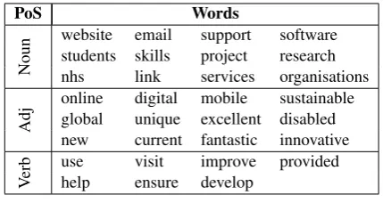
2billion tokens and4million types (Baroni et al., 2009).12 Therefore, a word-by-document model constructed from this corpus using the classic one-dimension-per-context-element method has a di-mension of2.69 million. In order to keep the ex-periments computationally tractable, the reported results are limited to 31 words from this model, which are listed in Table1.
In the designed experiment, a word from the list is taken as the reference and its`1 distance to the remaining 30 words is calculated using the vec-tor representations in the high-dimensional VSM. These 30 words are then sorted in ascending or-der by the calculated`1 distance. The procedure
is repeated for all the31words in the list, one by one. Therefore, the procedure results in31sorted lists, each containing30words. Figure2shows an example of the obtained sorted list, in which the reference is the word ‘research’.13
The procedure described above is replicated to obtain the lists of sorted words from VSMs that are constructed by the RMI method at reduced
11E.g. see the experiments inBullinaria and Levy (2007). 12UkWaC can be obtained from http://goo.gl/
3isfIE.
13Please note that the number of possible arrangements of 30words without repetition in a list in which the order is important (i.e. all permutations of30words) is30!.
PoS Words
Noun
website email support software students skills project research
nhs link services organisations
Adj
online digital mobile sustainable global unique excellent disabled new current fantastic innovative
Verb
use visit improve provided
[image:6.595.310.525.61.175.2]help ensure develop
Table 1: Words employed in the experiments.
nhs inno
vativesustainablefantasticglobal disabledmobiledigital improvedevelop unique organisationsexcellentlink softw
arecurrentskills ensure email visit provided online projectwebsitestudentsservicessupporthelp use new
Figure 2: List of words sorted by their`1 distance
to the word ‘research’. The distance increases from left to right and top to bottom.
dimensionality, when the method’s parameters— i.e. the dimensionality of VSM and the number of non-zero elements in index vectors—are set dif-ferently. We expect the obtained relative `1 dis-tances between each reference word and the 30
other words in an RMI-constructed VSM to be the same as the obtained relative distances in the orig-inal high-dimensional VSM. Therefore, for each VSM that is constructed by the RMI technique, the resulting sorted lists of words are compared by the sorted lists that are obtained from the original high-dimensional VSM.
We employ theSpearman’s rank correlation co-efficient (ρ) to compare the sorted lists of words and thus the degree of distance preservation in the RMI-constructed VSMs at reduced dimensional-ity. The Spearman’s rank correlation measures the strength of association between two ranked vari-ables, i.e. two lists of sorted words in our experi-ments. Given a list of sorted words obtained from the original high-dimensional VSM (listo) and its
corresponding list obtained from a VSM of re-duced dimensionality (listRMI), the Spearman’s
rank correlation for the two lists is calculated by
ρ= 1− 6
P d2
i
n(n2−1), (11)
wherediis the difference in paired ranks of words
in listo and listRMI, and n = 30 is the number
of words in each list. We report the average ofρ
100 200
400 800
1600 3200 48 16
32
64 0.5
0.7 0.91
dimension
|non-zero elements
|
¯
ρ
0.4 0.6 0.8 ¯
[image:7.595.101.262.63.207.2]ρ
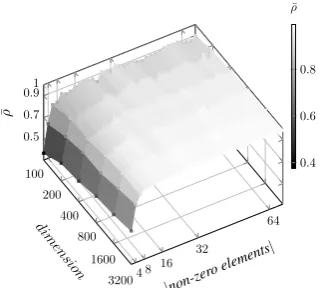
Figure 3: Theρ¯axis shows the observed average Spearman’ rank correlation between the order of the words in the lists that are sorted by the`1
dis-tance obtained from the original high-dimensional VSM and the VSMs that are constructed by RMI at reduced dimensionality using index vectors of various numbers of non-zero elements.
indicate the performance of RMI with respect to its ability for distance preservation. The closerρ¯
is to 1, the better the performance of RMI. Figure3shows the observed results at a glance when the distances are estimated using the median (Equation7). As shown in the figure, when the di-mension of the VSM is above400and the number of non-zero elements is more than12, the obtained relative distances from the VSMs constructed by the RMI technique start to be analogous to the rel-ative distances that are obtained from the origi-nal high-dimensioorigi-nal VSM, i.e. a high correlation (ρ >¯ 0.90). For the baseline, we report the av-erage correlation of ρ¯random = −0.004 between
the sorted lists of words obtained from the high-dimensional VSM and 31 ×1000lists of sorted words that are obtained by randomly assigned dis-tances.
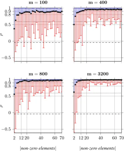
Figure 4 shows the same results as Figure 3, however, in minute detail and only for VSMs of dimension m ∈ {100,400,800,3200}. In these plots, squares ( ) indicate theρ¯while the error bars show the best and the worst observed ρ amongst all the sorted lists of words. The minimum value of ρ-axis is set to 0.611, which is the worst ob-served correlation in the baseline (i.e. randomly generated distances). The dotted line (ρ = .591) shows the best observed correlation in the baseline and the dashed-dotted line shows the average cor-relation in the baseline (ρ = −0.004). As sug-gested in Section 2.2, it can be verified that an
increase in the dimension of VSMs (i.e. m) in-creases the stability of the obtained results (i.e. the probability of preserving distances increases). Therefore, for large values ofm (i.e.m > 400), the difference between the best and the worst ob-servedρdecreases; average correlationρ¯→1and the observed relative distances in RMI-constructed VSMs tend to be identical to those in the original high-dimensional VSM.
Figure 5 represents the obtained results in the same setting as above, however, when the dis-tances are approximated using the geometric mean (Equation10). The obtained average correlations
¯
ρ from the geometric mean estimations are al-most identical to the median estimations. How-ever, as expected, the geometric mean estimations are more reliable for small values ofm; particu-larly, the worst observed correlations when using the geometric mean are higher than those observed when using the median estimator.
−0.5 0 0.5 1 0.8 0.9
ρ
m=100 m=400
20 40 60
−0.5 0 0.5 1
2 12 70
0.8 0.9
|non-zero elements|
ρ
m=800
20 40 60
2 12 70
|non-zero elements|
m=3200
Figure 4: Detailed observation of the ob-tained correlation between relative distances in RMI-constructed VSMs and the original high-dimensional VSM. The `1 distance is estimated
−0.5 0 0.5 1 0.8 0.9
ρ
m=100 m=400
20 40 60
−0.5 0 0.5 1
2 12 70
0.8 0.9
|non-zero elements|
ρ
m=800
20 40 60
2 12 70
|non-zero elements|
[image:8.595.86.287.64.310.2]m=3200
Figure 5: The observed results when the `1
dis-tance in RMI-constructed VSMs is estimated us-ing the geometric mean.
3 Random Manhattan Integer Indexing
The application of the RMI method is hindered by two obstacles: float arithmetic operations required for the construction and processing of the RMI-constructed VSMs and the calculation of the prod-uct of large numbers when `1 distances are
esti-mated using the geometric mean.
The proposed method for the generation of in-dex vectors in RMI results in inin-dex vectors of non-zero elements that are real numbers. Conse-quently, index vectors and thus context vectors are arrays of floating point numbers. These vectors must be stored and accessed efficiently when using the RMI technique. However, resources that are required for the storage and processing of floating numbers is high. Even if the requirement for the storage of index vectors is alleviated, e.g., using a derandomization technique for their generation, context vectors that are derived from these index vectors are still arrays of float numbers. To tackle this problem, we suggest substituting the value of non-zero elements of RMI’s index vectors (given in Equation6) from U1 to integer values of bU1c, whereb1
Uc 6= 0. We argue that the resulting
ran-dom projection matrix still has a Cauchy distribu-tion. Therefore, the proposed methodology to esti-mate the`1distance between vectors is also valid.
The `1 distance between context vectors must
be estimated using either the median or the geo-metric mean. The use of the median estimator— for the reasons stated in Section2.1—is not plau-sible. On the other hand, the computation of the geometric mean can be laborious as the overflow is highly likely to happen during its computation. Using the value ofb1
Ucfor non-zero elements of
index vectors, we know that for any pair of context vectors~u= (u1,· · · , um)and~v= (v1,· · · , vm),
ifui 6=vi then|ui−vi| ≥1. Therefore, forui 6= vi,ln|ui−vi| ≥0and thusPmi=1ln(|ui−vi|)≥0. In this case, the exponent in Equation10is a scale factor that can be discarded without a change in the relative distances between vectors.14 Based on the intuition that the distance between a vector and itself is zero and the explanation given above, in-spired by smoothing techniques and without being able to provide mathematical proofs, we suggest estimating the relative distances between vectors using
ˆ
L1(~u,~v) = m X
i=1 ui6=vi
ln(|ui−vi|). (12)
In order to distinguish the above changes in RMI, we name the resulting technique random Manhat-tan integer indexing (RMII). The experiment de-scribed in Section2.2is repeated using the RMII method. As shown in Figure6, the obtained results are almost identical to the observed results when using the RMI technique. While RMI performs slightly better than RMII in lower dimensions, e.g.
m= 400, RMII shows more stable behaviour than RMI at higher dimensions, e.g.m= 800.
4 Comparison of RMI and RI
RMI and RI utilize a similar two-step procedure consisting of the creation of index vectors and the construction of context vectors. Both methods are incremental techniques that construct a VSM at reduced dimensionality directly, without requiring the VSM to be constructed at its original high di-mension. Despite these similarities, RMI and RI are motivated by different applications and
math-14Please note that according to the axioms in the distance
definition, the distance between two numbers is always a non-negative value. When index vectors consist of non-zero ele-ments of real numbers, the value of|ui−vi|can be between
0 and 1, i.e.0<|ui−vi|<1. Therefore,ln(|ui−vi|)can
−0.5 0 0.5 1 0.8 0.9
ρ
m=100 m=400
20 40 60
−0.5 0 0.5 1
2 12 70
0.8 0.9
|non-zero elements|
ρ
m=800
20 40 60
2 12 70
|non-zero elements|
[image:9.595.87.286.63.310.2]m=3200
Figure 6: The observed results when using the RMII method for the construction and estimation of the`1distances between vectors. The method is evaluated in the same setup as the RMI technique.
ematical theorems. As described above, RMI ap-proximates the`1distance using anon-linear esti-mator, which has not yet been employed for the construction of VSMs and the calculation of `1
distances in distributional approaches to seman-tics. Moreover, RMI is justified using Cauchy ran-dom projections.
In contrast, RI approximates the`2 distance
us-ing a linear estimator. RI has initially been justi-fied using the mathematical model of the sparse distributed memory (SDM)15. Later, Sahlgren (2005) delineates the RI method using the lemma proposed byJohnson and Lindenstrauss (1984)— which elucidates random projections in Euclidean spaces—and the reported refinement inAchlioptas (2001) for the projections employed in the lemma. Although both the RMI and RI methods can be established as α-stable random projections— respectively for α = 1 and α = 2—the meth-ods cannot be compared as they address different goals. If, for a given task, the`1norm outperforms
the `2 norm, then RMI is preferable to RI. Con-trariwise, if the`2 norm outperforms the`1 norm,
then RI is preferable to RMI.
To support the earlier claim that RI-constructed
15SeeKanerva (1993) for an overview of the SDM model.
−0.5 0 0.5 1 0.8 0.9
ρ
m=400, the`1distance m=800, the`1distance
20 40 60
−0.5 0 0.5 1
2 12 70
0.8 0.9
|non-zero elements|
ρ
m=400, median estimator
20 40 60
2 12 70
|non-zero elements|
[image:9.595.322.521.64.310.2]m=800, median estimator
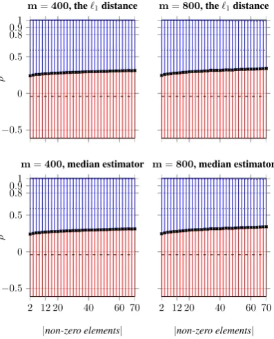
Figure 7: Evaluation of RI for the`1distance
esti-mation form = 400andm = 800when the dis-tances are calculated using the standard definition of distance in`1normed spaces and the median
es-timator. The obtained results using RI do not show correlation to the`1distances in the original
high-dimensional VSM.
VSMs cannot be used for the`1 distance
estima-tion, we evaluate the RI method in the experimen-tal setup that has been used for the evaluation of RMI and RMII. In these experiments, however, we use RI to construct vector spaces at reduced dimensionality and estimate the `1 distance
us-ing Equation 5 (the standard `1 distance
defini-tion) and Equation 7 (the median estimator) for
m ∈ 400,800. As shown in Figure7, the experi-ments support the theoretical claims.
5 Conclusion
In this paper, we introduce a novel technique, named Random Manhattan Indexing (RMI), for the construction of `1 normed VSMs directly at
reduced dimensionality. We further suggest the Random Manhattan Integer Indexing (RMII) tech-nique, a computationally enhanced version of the RMI technique. We demonstrated the`1 distance
dimensionality of the VSM, influence the obtained results. The proposed incremental (and thus effi-cient and scalable) methods significantly enhance the computation of the`1distances in VSMs.
Acknowledgements
This publication has emanated from research conducted with the financial support of Sci-ence Foundation Ireland under Grant Number SFI/12/RC/2289.
References
[Achlioptas2001] Dimitris Achlioptas. 2001. Database-friendly random projections. In Pro-ceedings of the Twentieth ACM SIGMOD-SIGACT-SIGART Symposium on Principles of Database Systems, PODS ’01, pages 274–281, New York, NY, USA. ACM.
[Baroni et al.2009] Marco Baroni, Silvia Bernardini, Adriano Ferraresi, and Eros Zanchetta. 2009. The wacky wide web: a collection of very large linguis-tically processed web-crawled corpora. Language Resources and Evaluation, 43(3):209–226.
[Brand2006] Matthew Brand. 2006. Fast low-rank modifications of the thin singular value decom-position. Linear Algebra and its Applications, 415(1):20–30. Special Issue on Large Scale Linear and Nonlinear Eigenvalue Problems.
[Brinkman and Charikar2005] Bo Brinkman and Moses Charikar. 2005. On the impossibility of dimension reduction in l1. J. ACM, 52(5):766–788.
[Bullinaria and Levy2007] John A. Bullinaria and Joseph P. Levy. 2007. Extracting semantic repre-sentations from word co-occurrence statistics: A computational study. Behavior Research Methods, 39:510–526.
[Deerwester et al.1990] Scott C. Deerwester, Susan T. Dumais, Thomas K. Landauer, George W. Furnas, and Richard A. Harshman. 1990. Indexing by latent semantic analysis. Journal of the American Society of Information Science, 41(6):391–407.
[Indyk2000] Piotr Indyk. 2000. Stable distribu-tions, pseudorandom generators, embeddings and data stream computation. In Foundations of Com-puter Science, 2000. Proceedings. 41st Annual Sym-posium on, pages 189–197.
[Indyk2006] Piotr Indyk. 2006. Stable distributions, pseudorandom generators, embeddings, and data stream computation. J. ACM, 53(3):307–323, May. [Johnson and Lindenstrauss1984] William Johnson and
Joram Lindenstrauss. 1984. Extensions of Lips-chitz mappings into a Hilbert space. InConference in modern analysis and probability (New Haven,
Conn., 1982), volume 26 ofContemporary Mathe-matics, pages 189–206. American Mathematical So-ciety.
[Kanerva et al.2000] Pentti Kanerva, Jan Kristoferson, and Anders Holst. 2000. Random indexing of text samples for latent semantic analysis. In Proceed-ings of the 22nd Annual Conference of the Cognitive Science Society, pages 103–6. Erlbaum.
[Kanerva1993] Pentti Kanerva. 1993. Sparse dis-tributed memory and related models. In Mo-hamad H. Hassoun, editor,Associative neural mem-ories: theory and implementation, chapter 3, pages 50–76. Oxford University Press, Inc., New York, NY, USA.
[Ke and Kanade2003] Qifa Ke and Takeo Kanade. 2003. Robust subspace computation using`1norm.
Technical Report CMU-CS-03-172, School of Com-puter Science, Carnegie Mellon University.
[Kwak2008] Nojun Kwak. 2008. Principal component analysis based on l1-norm maximization. Pattern Analysis and Machine Intelligence, IEEE Transac-tions on, 30(9):1672–1680, Sept.
[Lee1999] Lillian Lee. 1999. Measures of distribu-tional similarity. In Proceedings of the 37th An-nual Meeting of the Association for Computational Linguistics on Computational Linguistics, ACL ’99, pages 25–32, Stroudsburg, PA, USA. Association for Computational Linguistics.
[Lenci2008] Alessandro Lenci. 2008. Distributional semantics in linguistic and cognitive research. From context to meaning: Distributional models of the lex-icon in linguistics and cognitive science, special is-sue of the Italian Journal of Linguistics, 20/1:1–31. [Li et al.2007] Ping Li, Trevor J. Hastie, and
Ken-neth W. Church. 2007. Nonlinear estimators and tail bounds for dimension reduction inL1using cauchy
random projections. J. Mach. Learn. Res., 8:2497– 2532.
[Li2007] Ping Li. 2007. Very sparse stable random projections for dimension reduction inlα(0< α <
2)norm. InProceedings of the 13th ACM SIGKDD International Conference on Knowledge Discovery and Data Mining, KDD ’07, pages 440–449, New York, NY, USA. ACM.
[Li2008] Ping Li. 2008. Estimators and tail bounds for dimension reduction in`α(0 < α ≤ 2)using sta-ble random projections. InProceedings of the Nine-teenth Annual ACM-SIAM Symposium on Discrete Algorithms, SODA ’08, pages 10–19, Philadelphia, PA, USA. Society for Industrial and Applied Math-ematics.
[Sahlgren2005] Magnus Sahlgren. 2005. An introduc-tion to random indexing. InMethods and Applica-tions of Semantic Indexing Workshop at the 7th In-ternational Conference on Terminology and Knowl-edge Engineering, TKE 2005.
[Turney and Pantel2010] Peter D. Turney and Patrick Pantel. 2010. From frequency to meaning: vec-tor space models of semantics. J. Artif. Int. Res., 37(1):141–188, January.