Abstract—Face recognition has been of interest to a growing number of researchers due to its applications on security. Within past years, numerous face recognition algorithms have been proposed by researchers. However, there is no evidence that shows one specific proposed method is the best under all circumstances. So, a combination of several methods can be a good approach. Committee machine structures, which were introduced in the machine learning community, show some ways to combine different methods in a single framework. A committee machine structure makes decision according to its components. In the previous face recognition methods with committee machines, only the information which is extracted from test phase is used for combining classifiers. In this paper, in addition to the information in test phase, training phase information is used for combining classifiers. For this purpose, we introduce a new unit which is called “Region Finder”. This unit is attached to each classifier in a committee machine structure and is learned based on train phase information. A region finder determines its classifier recognition power in the classifier feature space. We applied our idea to a structure of five well-known classifiers, PCA, ICA, LDA, SVM and neural networks which are implemented for face recognition. Comparative experimental results of our committee machine with different algorithms and the structure without region finder units, demonstrate that the proposed system achieves improved accuracy.
Index Terms— Face Recognition, Committee Machine, Region Finder, Combining Several Classifiers.
I. INTRODUCTION
FACE RECOGNITION (FR) has a wide range of applications, such as face-based video indexing and browsing engines, biometric identity authentication, human-computer interaction, and multimedia monitoring/surveillance. Within the past two decades, numerous FR algorithms have been proposed, and detailed surveys of the developments in the area have appeared in the literature [1].
Among various FR methodologies used, the most popular are the so-called appearance-based approaches, which include the four most well-known FR methods, namely Eigenfaces [2], Fisherfaces [3], Bayes Matching [4] and ICA [5]. With focus on low-dimensional statistical feature extraction, the appearance-based approaches generally operate directly on appearance images of face object and process them as two-dimensional (2-D) holistic patterns to avoid difficulties
associated with three-dimensional (3-D) modeling [6], and shape or landmark detection [7].
Although there are several algorithms for face recognition, but there is no evidence which shows one of them, is the best one under all circumstances [8] [9]. In addition to this fact, our experiments revealed that one method may not be able to recognize a test face correctly; while a lower recognition rate method on the same database can recognize it correctly.
These two reasons are a good motivation for us to combine several FR methods. The most important issue that should be considered in each combination of several methods is that: every method of a combination should keep its own power and try to compensate other methods weakness.
In recent years, the committee machine, an ensemble of estimators, has proven to give more accurate results than the use of a single predictor. The basic idea is to train a committee of estimators and combine the individual predictions to achieve improved generalization performance. Different approaches are proposed by researchers within the last ten years [10]. There exist two types of structure [11]:
1. Static Structure: This is generally known as an
ensemble method. Input data is not involved in combining the committee experts. Examples include ensemble averaging and boosting.
2. Dynamic Structure: Input is directly involved in the
combining mechanism that employs an integrating unit to adjust the weight of each expert according to the input.
Recently, researchers have applied the committee machine in various fields. In face recognition, Gutta et al. used an ensemble of Radial Basis Function (RBF) network and a decision tree in the face processing problem [12] [13]. Huang et al. formulated an ensemble of neural networks for pose invariant face recognition [14].
Generally, two kinds of committee machine structures have been introduced for FR. The first one uses a structure of similar classifiers which each of them is learned on a subset of the train set. On the other hand, the second structure contains several different classifiers and uses whole of the train set for learning each classifier. In this paper, we propose a solution to improve the second category of FR committee machine structures with introducing a new unit which is called “Region Finder”.
A Solution of Combining Several Classifiers for
Face Recognition
Table 1: An example of a “similarity table”. This table shows the result of testing the train faces with a PCA classifier which has been learned on these train faces before. The values in parenthesis show classes of instances. The distances between each instance to the train instance (column 1)
is placed in the second raw of each case.
The rest of this paper is organized as follows: Section 2 describes some previous combined methods for face recognition. Section 3 introduces region finder units. Section 4 presents our proposed structure. Section 5 reports experimental results and finally section 6 provides a conclusion.
II. PREVIOUS WORKS
There are basically two classifier combination scenarios for FR. In the first scenario, all the classifiers use the same representation of the input pattern. A typical example of this category is a set of LDA classifiers that are arranged in a structure with the AdaBoost algorithm [15][16]. In the second scenario, each classifier uses its own representation of the input pattern. In other words, several classifiers, each of them is a well-known FR method, are combined in this approaches.
In this paper, we focus on classifier combination in the second scenario. According to ways that are used for combining classifiers result to obtain a final result, several approaches have been proposed.
In reference [17], some combination schemes such as the product rule, sum rule, min rule, max rule, mean rule, and majority voting are introduced. These methods use probability and the bayes theorem for combing classifiers. In reference [18] some different arrangements of five classifiers are combined with the mean rule.
FR committee machines are another methods of the second category. These methods usually use voting or weighted voting mechanisms for combing classifiers. References [19], [20] introduced a structure of five FR classifiers (PCA, LDA, EGB, SVM, and NN). In the train phase, each classifier is learned on the train set individually. In the test phase, first each classifier determines its result; then the structure calculates beliefs for each result. A result with the greatest belief will be selected as the structure result. The beliefs are calculated according to information in test phases. For example, for PCA, ICA, and LDA classifiers, beliefs are calculated with counting the number of similar recognized faces in the first five results.
For getting best combination results, we should use the most information which can be extracted. In the mentioned structures, information which lies in train phase is ignored for calculating the beliefs. We are going to use this information for improving the results. For this purpose, a new unit which is called “Region finder” will be introduced. This unit is attached to each classifier and calculates a base belief for the classifier results according to the classifier train phase information.
III. REGION FINDERS
Region finder is a learning agenda which is assigned to each classifier in a committee machine structure. This unit indicates distribution of the classifier recognition power in the classifier feature space. A region finder is learned in its classifier train phase. In test phase, it calculates a base belief for its classifier result according to the location of the test instance in the classifier feature space. For example, if a classifier has a high recognition power in a subspace of its feature space and a test instance locates in this area, the belief to the classifier result for this test instance is high.
For explaining how a region finder is learned in train phase, consider the table 1. This table, which we call it a “similarity table”, shows the results of testing the train instances with a classifier that has been learned on these train instances before. With consideration to table 1, the following results can be exploited.
According to the first row: the train instance 57 (class=12)
and 101 (class=21) are nearer to the train instance 1 (class=1) than train instance 2 (class=1). So there are two train instances whose classes are not 1 (instances 57 and 101) but are more similar to train instance 1 rather than some instances of class 1 (instances 3, 2, and 5). Based on similarities between instances 1, 57, and 101, they may make some difficulties for each other in recognition. For example, suppose there is a test instance of class 1 and the most similar train face of class 1 to it, is face 1. If it is given to this classifier, the classifier may result class 12 or 13 instead of class 1. Therefore it can be said that the classifier Train
Instance
first near
instance
Second near
instance
Third near
instance
Fourth near
instance
Fifth near
instance
Sixth near
instance
1(1) 1(1)
0.0
57(12) 0.03
3 (1) 0.14
101(21) 0.16
2(1) 0.17
5(1) 0.21
2(1) 2 (1)
0.0
3(1) 0.03
1(1) 0.09
179(36) 0.12
22(5) 0.15
137(28) 0.17
7(2) 7(2)
0.0
10(2) 0.01
9(2) 0.03
8(2) 0.05
6(2)
0.05
78(16) 0.22
200(40) 200(40)
0.0
132(27) 0.11
57(12) 0.17
59(12) 0.21
196(40) 0.22
does not have a good recognition power in these instances.
According to the third row: Recognition power of this
classifier in the instance 7 (class=2) is high. The first reason is that other instances of class 2 are the nearest instances to it. The second reason is related to distances class 2 and non-class 2 instances to instance 7. Instance 78 (class=16) as the nearest non-class 2 instance is so far from instance 7. That indicates that all instances which are belong to class 2 have a small distance to each other and their distances to other instances are high. According to these two reasons, the classifier can correctly recognize test instances that are placed near to instance 7.
According to the first and fourth rows: Recognition power
of the classifier in instance 57 (class=12) is low. This instance is near to at least two instances (1 and 200) from other classes. So if the classifier makes a decision about a test instance that is near to instance 57, we will not be sure about the correct class.
In the following section, we describe some measures which are defined on each row of a similarity table. These measures are used for estimating a classifier recognition power in the classifier feature space.
IV. FACE RECOGNITION COMMITTEE MACHINE WITH REGION FINDERS UNITS
Our proposed face recognition structure is shown in the Fig 1. There are five different classifiers with their region finders in the structure. Also there is a gating network unit which extracts final results. In the following, each section of the structure is described.
A. Classifiers and their region finder
Five different classifiers (PCA, ICA, LDA, SVM, and NN) are trained individually on the train set in the first phase of training. Some comments about these classifiers are:
- The PCA classifier uses 30 first principal components of each train and test face as their feature vector.
- The SVM and NN classifiers use raw image gray values as input for training.
- The NN classifier is a back propagation neural network. - The SVM classifier uses one-against-one method for
classification.
Second phase of training is related to learn region finders. A region finder that is assigned to a classifier, which has been learned with train instances before, is learned as following: 1) Give train faces as test faces to the classifier.
2) For each train face, information about its similarities to other train faces is extracted and shown in a similarity table.
3) According to each classifier characteristics, some measures are defined on the similarity table. These measures are shown in tables 2-5 and will be discussed later.
4) Measure values are normalized according to their mode (positive: high values of these measures indicate high
recognition power and vice versa for the negative mode) with (1) and (2).
) ( )
(
) ( )
(
i Average i
Maximum
i Measure i
Maximum −
− (1)
) ( )
(
) ( )
(
i Minimum i
Average
i Measure i
Average −
− (2)
Equation (1) is applied to the positive mode measures and (2) for negative ones. By using these relations, a set of measures values in (-1, +1) are calculated for each train instance.
5)
For assigning a single value to each train instance which indicates the classifier recognition power on it, a weighted average of its normalized measure values is needed. For simplicity, we assume all the measures have an equal weight in the average (3).∑
== mk
j k
i mv i j
m k n
power( , ) 1 1 ( , ) (3)
In (3), power (ni, k) stands for the recognition power of kth
classifier to ith train instance and mv(i,j) is the jth normalized measure value for ith train instance. Also mk is the number of
measures that are defined for kth classifier.
6)
For each train instance, its feature vector (according to a classifier feature space) and the classifier recognition power on it, are given to the region finder. (In our structure a region finder is a neural network that uses these values as inputs and outputs for learning.)In the following, mentioned measures are described for each classifier separately.
[image:3.595.314.539.605.712.2]PCA and ICA: These measures are shown in table 2. We assume that there are k train faces for each person in the data set and these classifiers use K-nearest neighbor method for finding similar train instances to each test sample. A “result” in table 2 refers to a train face from the K nearest train faces. (Remember that these measures apply on results of testing the train faces. So test faces and train faces are the same in this step). Also a “positive situation” refers to be in the first K nearest instances to a test face with a similar class. For example in table 1, in the second row instance 1 has a positive situation and instance 132 in the forth row has a negative situation.
Table 2: Measures for learning region finders in PCA and ICA classifiers
Measure Description Mode
1 Number of correct recognized results in the first K
results +
2 The first incorrect result index +
3 Distance between the first correct and the first
incorrect result +
4 Distance between the first incorrect result and its
previous +
5 Number of times that the instance is placed in a
positive situations +
6 Number of times that the instance is placed in a
negative situations -
Fig 1: The schematic view of our face recognition committee machine structure
LDA: According to the supervised learning methodology which is used in this classifier, some measures which have been introduced for PCA and ICA can not be useful here. It is happened because LDA sets all instances of a class as the nearest instances in its feature space. LDA measures are shown in table 3.
If there are K train instances for each class, a train face which locates in position K+1 in the similarity table, is assumed as a candidate result. For example in table 1, instance 78 is a candidate result in row 3.
SVM, NN:Although measures that are used for these two classifiers are similar, but their descriptions are different. In SVM to recognize a test image in J different classes, J*(J-1)/2 SVMs are constructed. The image is tested against each SVM and the class with the highest votes in all SVMs is selected as the result. A “distance” for an instance is equal to sum of distances between its SVMs value and the winner class. These distances will be normalized with dividing by number of SVMs.
In the Neural Network classifier, we choose a binary vector of size J for the target representation. The target class is set to one and others are set to zero. The class whose output value is the closest to 1 is chosen as the result and the output value is chosen as its “normalized distance”. These measures for SVM and NN can be found in tables (3)-(4).
Table 3: Measures for learning region finders in LDA classifiers
Measure Description Mode
1 Distance between the first correct and the first incorrect result + 2 Distance between the first incorrect result
and its previous +
3 Distance between the first and the last
correct results +
4 Number of times that the instance is placed as a candidate result -
Table 4: Measures for learning region finders in the SVM and NN classifiers
Measure Description Mode
1 Normalized distance for the first winner + 2 Difference between the first and second
winner +
3 Number of times that the instance is placed as a candidate results -
B. The gating network
This unit is active in the test phase and gets the classifiers result as input and gives the final structure result as its output. It has three sections:
- Calculate base beliefs:This section gets a test instance and
converts it to each classifier feature space, then gives this converted feature vector to classifier region finders. Region finders output indicate base beliefs for each classifier result.
- Adjust base beliefs:Remember that we want to use both the
test and train phases information for combining classifier. This section calculates a confidence for each classifier result based on test phase information. Similar to calculate base beliefs, these confidences are defined specifically for each classifier and are as following:
PCA, ICA, and LDA: Confidence for a result is the number of votes which the result gets among the K first results (4).
K i r v i
c( ) = ( ( )) (4)
SVM: Its confidence is defined by the votes which the result yields between all the SVMs (5).
1 )) ( ( ) (
− =
J i r v i
c (5)
NN: The neural network output value, which indicates the result, is its confidence too.
finally J is the number of train classes. After calculating base beliefs and confidences for a test instance i, final beliefs to each classifier result is got according to (6).
belief
(
i
)
=
base
_
belief
(
i
)
×
confidence
(
i
)
(6)- Find final result and its belief: The gating network selects
the result that has the highest belief as the final result. Also the final result’s belief is assumed as the structure belief to its result.
V. EXPERIMENTS AND RESULTS
For evaluating the performance of our proposed structure, we set some experiments which each of them evaluates one aspect of our method.
A. Data Set
All the tests have been conducted on the ORL dataset [21], the Yale dataset [22], and the Yale-B dataset [23] which are three of the most used benchmarks in this field. ORL consists of 400 different images related to 40 individuals. The Yale database contains 165 faces of 15 persons. Eleven different facial expressions are assumed for each person. Yale-B contains of 5760 single light source images of 10 individuals each seen under 576 different viewing conditions (poses and illumination conditions).
For all experiments (Except section D), we divided each dataset randomly and uniformly to a train set and a test set (For example, in the ORL dataset, we used 5 images per person as a training set and then we tested the algorithm on the 5 remaining images.). For all the datasets, to minimize the possible misleading results caused by the training data, the results have been averaged over ten experiments.
B. Evaluating the structure performance
A combined method will be called an efficient structure if its performance is higher than methods which contribute in the combination. We applied our structure and its component methods to our data sets. The results are shown in table 5. It can be seen easily that our structure has higher performances than its components.
Table 5: Compare our structure performance with its five classifiers Dataset PCA ICA LDA SVM NN Our
Structure
ORL 0.88 0.87 0.93 0.91 0.84 0.97
Yale 0.66 0.76 0.82 0.79 0.77 0.91
YaleB 0.75 0.81 0.88 0.89 0.84 0.92
C. Comparing our structure with some other fusion methods
In this section, we want to compare our method with some other methods which have been proposed for combining classifiers. This comparison is shown in table 6. These algorithms are implemented according to their references and
with the same classifiers as our proposed structure. These results demonstrate that our proposed method usually outperforms these fusion methods.
D. Evaluating the effect of training face number on the performance
[image:5.595.300.555.295.407.2]Usually, FR classifier’s performance and the number of training faces have a direct relationship to each other. When the number of training faces decreases, classifier’s performance will decrease too. We want to compare this effect on our structure and its components. We examined them on 9 couples of train/test sets which are built from the ORL. They are different in the dataset division rate. The results, which are shown in table 7, demonstrate our approach is more reliable to decrement in training faces.
Table 7: Compare our proposed method and its component in different division rate.
Set PCA ICA LDA SVM NN Our Structure
10% test 0.9 0.87 0.96 0.95 0.92 0.99
20% test 0.87 0.86 0.96 0.94 0.91 0.99
30% test 0.89 0.90 0.94 0.94 0.90 0.98
40% test 0.85 0.85 0.93 0.92 0.90 0.96
50% test 0.88 0.87 0.92 0.91 0.82 0.95
60% test 0.81 0.79 0.86 0.87 0.74 0.91
70% test 0.73 0.72 0.81 0.80 0.70 0.84
80% test 0.71 0.71 0.74 0.75 0.63 0.80
90% test 0.62 0.64 0.58 0.67 0.51 0.76
E. Evaluating the region finders roll in the structure
We suggest region finder units, which contribute train phase information in the combination of classifier results, to be attached to common face recognition committee machines. For evaluating this suggestion, we compared two structures:
Structure 1: The proposed committee machine structure. Structure 2: A structure that is similar to the first one, except
[image:5.595.321.534.587.637.2]that it dose not have region finder units. In this structure, a belief for each classifier result is calculated only according to test phase information (belief (i) =confidence (i) in (6)). The comparison between these two structures on our datasets is shown in table 8. The results show that region finders make higher the performance about 5%.
Table 8: The comparison between structure 1 and structure 2. Set Structure 1 Structure 2
ORL 0.958 0.909
Yale 0.91 0.87
YaleB 0.92 0.85
F. Evaluating the maximum performance can be obtained with this structure
Table 6: Compare our proposed method with some other fusion methods Dataset Majority Vote
Rule[17]
Max Rule[17] Sum Rule[17] SFRCM[19] DFRCM[20] Our Structure
ORL 0.91 0.93 0.97 0.89 0.92 0.97
Yale 0.84 0.89 0.90 0.88 0.89 0.91
YaleB 0.85 0.88 0.90 0.87 0.90 0.92
[image:6.595.76.266.282.334.2]
We call a structure as an “ideal structure", if it can recognize a test instance correctly even one classifier in its structure can do it correctly. A comparison between our structure and an ideal structure with the same classifiers is shown in table 9. The results show our structure is near to its ideal structure. Also it seems with better region finders, our structure can achieve to its ideal version.
Table 9: Comparison between our proposed structure and the ideal version of it.
Dataset Ideal structure
performance Our structure performance
ORL 0.975 0.96
Yale 0.93 0.91
Yale-B 0.94 0.92
G. Structure belief to recognized and not recognized instances
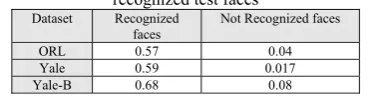
Our proposed structure has an additional property in compare to single classifier and previous committee machine mechanism. It can assign an accurate belief to each structure result. So if the classifier not be able to recognize a face correctly, it can be found with consideration to the assigned belief. In table 10, we calculated the average of result beliefs for recognized and not-recognized faces on our datasets. This property gives an extra opportunity to use other mechanism for judging about the low belief test instances.
Table 10: The average of the structure beliefs for recognized and not recognized test faces
Dataset Recognized
faces Not Recognized faces
ORL 0.57 0.04
Yale 0.59 0.017
Yale-B 0.68 0.08
VI. CONCLUSION AND FUTURE WORKS
In the proposed structure, we defined a mechanism to use information in the both train and test phases for combining classifiers result. Theoretically, it can be possible to get a structure whose performance is equal to one by using some independent methods (When union of recognized instances in a set of independent methods is equal to the test set). In addition to use independent methods, perfect region finders must be defined for this purpose. In the future, we are going to evaluate some other methods in our structures. Also we will try to improve the region finders, so we can achieve an ideal structure.
If several different methods proposed for an application, this committee machine structure has the ability to be applied on this application. So this can be an open area for future work.
REFERENCES
[1] W. Zhao, R. Chellappa, P. J. Phillips, and A. Rosenfeld,
“Face recognition: A literature survey”, ACM Computer
Survey, vol. 35, no. 4, 2003, pp. 399–458. [2] M. A. Turk and A. P. Pentland, “Eigenfaces for
recognition”, Journal of Neuroscience, vol. 3, no. 1, 1991,
pp. 71–86.
[3] P. N. Belhumeur, J. P. Hespanha, and D. J. Kriegman, “Eigenfaces vs. fisherfaces: Recognition using class specific linear projection”, IEEE Trans. Pattern Anal.
Mach. Intell., vol. 19, no. 7, 1997, pp. 711–720.
[4] B. Moghaddam, T. Jebara, and A. Pentland, “Bayesian face recognition”, Pattern Recognition, vol. 33, 2000, pp.
1771–1782.
[5] M. Bartlett, J. Movellan, and T. Sejnowski, “Face Recognition by Independent Component Analysis”, IEEE
Trans. on Neural Networks, Vol. 13, No. 6, 2002, pp. 1450-1464.
[6] V. Blanz and T. Vetter, “Face Recognition Based on Fitting a 3D Morphable Model”, IEEE Transactions on
Pattern Analysis and Machine Intelligence, Vol. 25, No. 9, 2003, pp. 1063-1074.
[7] L. Wiskott, J. Fellous, N. Krueuger, and C. Malsburg, “Face Recognition by Elastic Bunch Graph Matching”,
Chapter 11 in Intelligent Biometric Techniques in Fingerprint and Face Recognition, eds. L.C. Jain et al., CRC Press, 1999, pp. 355-396.
[8] K. Delac, M. Grgic, and P. Liatsis, “Appearance-based Statistical Methods for Face Recognition”, Croatian
Telecom conference, Savska 32, Zagreb, CROATIA, 1999.
[9] K. Delac, M. Grgic, S. Grgic, “A comparative study of PCA, ICA, and LDA”, Croatian Telecom conference,
Savska 34, Zagreb, Croatia,2001.
[10] Y. Freund and R. E. Schapire, “A short introduction to boosting”, Journal of Japanese Society for Artificial
Intelligence, 15, 1999, pp. 771-780.
[11] S. Haykin, “Neural Networks: A Comprehensive Foundation”, book, Prentice Hall PTR Upper Saddle
River, NJ, USA, 1998.
[12] S. Gutta, J. Huang, B. Takacs, and H. Wechsler “Face recognition using ensembles of networks”, In IEEE Proc.
13th International Conference on Pattern Recognition, volume 3, 1996, pages 50-54.
[13] S. Gutta, J. R. J. Huang, P. Jonathon, and H. Wechsler, “Mixture of experts for classification of gender, ethnic origin, and pose of human faces”, In IEEE Trans. on
Neural Networks, volume 11, 2000, pages 948-960. [14] F. J. Huang, H.-J. Zhang, T. Chen, and Z. Zhou, “Pose
[image:6.595.75.269.493.542.2]International Conference on Automatic Face and Gesture Recognition, 2000, pages 245-250.
[15] H. KONG, X. LI, W. Jian-Gang, and K. Chandra, “Ensemble LDA for face recognition”, International
conference on biometrics , Hong Kong, China, vol 3832, 2006, pp.166-172.
[16] J. Lu, K. Plataniotis, A. Venetsanopoulos, and S. Li, “Ensemble-Based Discriminant Learning With Boosting for Face Recognition”, IEEE transaction on neural
networks, Vol. 17, NO.1, 2006.
[17] J. Kittler, M. Hatef, R. Duin, and J. Matas, “On Combining Classifiers”, IEEE Trans. Pattern Anal. Mach. Intell., vol. 20, 1998, pp. 226–239.
[18] A. Lumini and L. Nanni, “Combining Classifiers To Obtain A Reliable Method For Face Recognition”, Special
Issue on Pattern Recognition in Biometrics and Bioinformatics, vol 3, no 3, 2005, pp. 47-53.
[19] H. Tang, M. Lyu, I. King, “Face recognition committee machine”, IEEE International Conference on Acoustics,
Speech, and Signal Processing, Vol.2, 2004, pp. 837-840. [20] H. Tang, M. Lyu, I. King, “Face recognition committee
machines: dynamic vs. static structures”, 12th IEEE
International Conference on Image Analysis and Processing, 2004, pp. 121- 126.
[21] ORL database available:
http://www.uk.research.att.com/facedatabase.html. [22] Yale database available:
http://cvc.yale.edu/projects/yalefaces.html. [23] Yale-B database available: