Abstract—Nonplanar trajectory optimization problem with advanced variable specific impulse magnetoplasma rocket (VASIMR) engine is studied. A newly developed method called Gauss Pseudospectral method is applied to the nonplanar trajectory optimization problem with VASIMR engine. Three representative trajectory optimization problems are solved. The first is an orbit raising problem from LEO to GEO; the second is a transfer from LEO to Sun synchronous orbit with large inclination change; the third is a transfer from LEO to Molniya orbit. These three problems demonstrate the ability of VASIMR and Gauss Pseudospectral method to deal with different kind of trajectory optimization problems. The results show that VASIMR engine can greatly increase the payload ratio for its large specific impulse and can be applied in different kinds of orbital transfer problems. It also demonstrates the Gauss Pseudospectral method is a powerful and effective method to deal with complicated trajectory optimization problems. Especially it can catch the proper switching structure without solving the difficult two point boundary problem. The purpose of this paper is trying to make a contribution to different kinds of orbital transfer with VASIMR engine using Gauss Pseudospectral method.
Index Terms—trajectory optimization, variable specific impulse, Gauss Pseudospectral method
I. INTRODUCTION
Although chemical rocket engines still act as the main role in present space missions, many future space propulsion systems have been proposed. One of these is the famous variable specific impulse magnetoplasma rocket (VASIMR) which is being developed at the Johnson Space Flight Center. A VASIMR is a high-power magnetoplasma engine. Its specific impulse can vary continuously between a minimum value (3000s) and a maximum value (30000s). A VASIMR engine gives continuous and variable thrust at constant power. A 10KW space demonstrator experiment has been completed and a 200MW VASIMR engine could be available by the year 2050.
Many researchers have finished many great works using variable specific impulse propulsion system. Kluever[1]
Manuscript received June 22, 2007.
Xingang Liang is with Harbin Institute of Technology, Harbin 150001 (e-mail: [email protected]).
Di Yang is with Harbin Institute of Technology, Harbin 150001 (e-mail: [email protected]).
studied the geostationary orbit transfer using specific impulse modulation. Sang-Yong Park and Kyu-Hong Choi[2] utilizing the VASIMR engine achieved fast intercept/rendezvous trajectory to Earth-crossing objects. Senent Juan et al[3] studied variable specific impulse transfer to unstable periodic orbits. Hans Seywald et al[4] studied fuel-optimal transfers between coplanar circular orbits using VASIMR engine.
Current numerical methods for solving trajectory optimization problems fall into two general categories: indirect methods and direct methods[5]. In indirect methods, the first order optimality conditions are derived using the Pontryagin minimum principle. These necessary conditions lead to a two-point-boundary-value problem (TPBVP). However, indirect methods have significant disadvantages. First, the necessary optimality conditions must be derived analytically, for complicated problems this derivation is non-trivial and fallible. Second, the radius of convergence is typically small because the initial costates are very sensitive to boundary conditions and switching function. and providing a good initial guess is very difficult. In direct methods, the optimal control problem is discretized at a set of time points. The discretized problem is then transcribed to a nonlinear programming problem (NLP) and the NLP is solved using an appropriate optimization method. It is easier to find a solution to the NLP than to find a solution to the TPBVP. Direct methods have a large radius of convergence and the switching structure does not need to be known. Direct methods are capable of solving a much wider range of complex problems. Famous optimal control software packages employ direct methods such as NASA’s OTIS and Boeing’s SOCS.
A newly developed method for optimal control, called Gauss Pseudospectral Method, is given by Benson[6]. And he has proved the optimality conditions from Gauss Pseudospectral method is equivalent to the discretized form of the first-order necessary conditions of the optimal control problem. In Gauss pseudospectral method, the state and control are discretized at a set of points called Gauss points and they are approximated using Lagrange interpolating polynomials. Gauss pseudospectral discretization leads to a discrete NLP that can be solved using an appropriate NLP algorithm. Some work have been done using Gauss Pseudospectal[7, 8, 9]. As far as the authors know, no application of Gauss Pseudospectral method in nonplanar trajectory optimization with VASIMR
Nonplanar Trajectory Optimization with
Variable Specific Impulse Engine Using Gauss
Pseudospectral Method
engine occured.
In this research, Gauss Pseudospectral method is applied to the trajectory optimization problem with VASIMR engine. Three representative problems are solved: The first is an orbital raising from LEO to GEO, which demonstrates the orbital raising ability of VASIMR; the second is a transfer problem from LEO to Sun synchronous orbit, which demonstrates the large inclination change ability of VASIMR; and the third is a transfer from LEO to Molniya, which demonstrate the ability of VASIMR to transfer to a general inclined elliptic orbit. All other transfer problems can be regarded as the combinations of these three representative transfer problems. The results show that 1) VASIMR engine can be applied in different kind of orbit transfer problems and it is suitable for future big payload flight mission because of its large range of specific impulse and 2) Gauss Pseudospectral method is a powerful and effective method to deal with complicated trajectory optimization problems, especially for the problems with discontinuous controls such as problems with unknown switching structure.
II. PROBLEM FORMULATIONS
A. VASIMR Engine Model
The VASIMR engine model is given. A VASIMR engine can output continuous and variable thrust at a constant power. The thrust is inversely proportional to the specific impulse. The relation between thrust and specific impulse of a VASIMR is
0
2 /( sp ) .
T= Pη I g (1)
Where T is thrust magnitude; P is input power; η is power efficiency; Isp is specific impulse and g0 is the earth
gravitational acceleration at sea level. The mass flow rate is calculated by
2 2
0 0
/( sp ) 2 /( sp ) .
m= −T I g = − Pη I g (2)
B. Orbit Motion Equations with Modified Equinoctial
Elements
Spacecraft orbit motion under continuous thrust is often studied by using Gauss’s planetary perturbation equations with the classical orbital elements as state variables. However, singularity occurs when eccentricity and orbit inclination equal (or one of them equals) zero. To eliminate the singularity, many researchers have given several sets of nonsingular orbital elements. One of them called modified equinoctial elements, denoted by p, f, g, h, k, L (p is different from P). Modified equinoctial elements can eliminate singularity except when orbit inclination equals 180°, and they can be used in elliptic orbit and hyperbolic orbit. Modified equinoctial elements are adopted as state variables of orbital motion in this paper. They can be obtained from classic orbit elements.
(
)
(
)
(
)
( )
( )
2 1 cos sin tan / 2 cos tan / 2 sinp a e
f e g e h i k i L ω ω ω υ = −
= + Ω
= + Ω
= Ω
= Ω
= Ω + +
(3)
Where a, e, i, Ω, ω, υ are classical orbital elements which denote semimajor, eccentricity, inclination, argument of perigee, right ascension of node and true anomaly, respectively.
The orbit motion equations using modified equinoctial elements are shown below.
(
)
(
)
(
)
(
)
0 0 0 2 0 2 2 2 1 cos [ sinsin cos 2
]
1 sin
[ cos
sin cos 2
+ ] cos 2 2 sin t sp r t n sp r t n sp n sp
p p P
p
w I g m
w L f
p
f L
w
h L k L g P
w I g m
w L g
p
g L
w
h L k L f P
w I g m
p s L P
h
w I g m
p s L
k η α μ α α μ η α α α μ η α η α μ μ = + + = + − − + + = − + − = = 0 2 0 2 2
sin cos 2
n sp
n sp
P
w I g m
w p h L k L P
L p
p w I g m
η α η μ α μ ⎛ ⎞ − = ⎜ ⎟ + ⎝ ⎠ (4)
Where w= +1 fcosL g+ sinL , s2 = +1 h2+k2, μ is the
earth gravitational constant, ( , , )T r t n
α α α is the unit vector along the thrust direction expressed in radial-tangential-normal coordinate system. m is spacecraft instant mass.
C. Trajectory Optimization with VSAIMR Engine
The performance index is to maximize the mass at the terminal time tf.
( )f min
J= −m t → (5)
For simplicity, (4) is rewritten as matrix form.
11 12 13 21 22 23 31 32 33
41 42 43 0 51 52 53
61 62 63
0 0 0 2 0 0 r t sp n
p B B B
f B B B
g B B B P
B B B
h I g m
B B B
k
B B B d
L α η α α ⎡ ⎤ ⎡ ⎤ ⎡ ⎤ ⎢ ⎥ ⎢ ⎥ ⎢ ⎥ ⎢ ⎥ ⎢ ⎥⎡ ⎤ ⎢ ⎥ ⎢ ⎥ ⎢ ⎥⎢ ⎥ ⎢ ⎥ ⎢ ⎥ =⎢ ⎥⎢ ⎥ +⎢ ⎥ ⎢ ⎥ ⎢ ⎥⎢ ⎥ ⎢ ⎥ ⎢ ⎥ ⎢ ⎥⎣ ⎦ ⎢ ⎥ ⎢ ⎥ ⎢ ⎥ ⎢ ⎥ ⎢ ⎥ ⎢⎣ ⎥⎦ ⎢ ⎥⎣ ⎦ ⎣ ⎦ (6) Namely, 0 2 . sp P I g m
η
=B ⋅ +D
α
Where x= (p, f, g, h, k, L)T. α =(α
r,αt,αn)T. Matrix B and D can be obtained from (4). Bij (i = 1, 2, 3, 4, 5, 6; j = 1, 2, 3) are elements of B and d is the only nonzero element of D.
The Hamiltonian function is defined form (7) and (2).
2 2 0 0 2 2 T L m sp sp P P H d
I g m I g
η λ λ η
=λ αB ⋅ + − ⋅ (8)
The costate equations are
0 2 0 2 2 T L sp T m sp
H P d
I g m
H P
m I g m
η λ η λ ∂ ∂ ∂ = − = − − ∂ ∂ ∂ ∂ = − = ∂ B B
λ λ α
λ α
x x x
(9)
Where λ =(λp, λf, λg, λh, λk, λL)T, are the costates corresponding to p, f, g, h, k, L, respectively and λm is the costate corresponding to m.
In the problem concerned in this paper, thethrust directionα and specific impulse Isp are control variables. According to optimal control theory, they should make the Hamiltonian function minimal.
The optimal thrust direction unit vector α is obtained by making the Hamiltonian function minimal with the constraint
1
T =
α α .
( )
T T T= − B
B
λ α
λ (10)
Substituting (10) into Hamiltonian function, it shows that the Hamiltonian function is a quadratic polynomial about 1/Isp. The optimal specific impulse can be easily obtained to make the Hamiltonian function minimal through some fundamental algebra knowledge.
, when , when , when
sp spmin spmax
sp spmax spmax
sp spmin spmin
I k I k I
I I k I
I I k I
⎧ = < <
⎪ = ≥ ⎨ ⎪ = ≤ ⎩ (11) Where 0 2 m T m k g λ = − B
λ (12)
Ispmin and Ispmax are specific impulse lower and upper limit respectively.
The switching function can be taken as
0 . T m sp S
m I g
λ
= λ B + (13)
And the power P is decided by 0 if 0
. if 0
max
P S
P P S
= <
⎧
⎨ = >
⎩
,
, (14)
Where Pmax is the maximum power of VASIMR engine. In the above contents, trajectory optimization problem with VASIMR engine is given and the optimal specific impulse conditions are derived.
Although the problem can be solved by solving the corresponding TPBVP consisting of the canonical equations, the boundary conditions and the transversality conditions using some numerical algorithms for TPBVP, it is because of two
disadvantages that solving TPBVP is not adopted in this research. The first is that the costates equations in (9) have very complicated form. Especially, ∂B/∂x is a 6 3 6× × matrix. Every one of the 108 elements is very complicated and derivation and input for these elements are boring and fallible. The second disadvantage is that solving a TPBVP is difficult work. Many researchers have showed that it is difficult to solve the TPBVP if the switching function must be satisfied.
In order to avoid the two main disadvantages mentioned above, a newly developed algorithm for optimal control, which is called Gauss Pseudospectral method, is adopted to solving the trajectory optimization with VASIMR engine.
III. GAUSS PSEUDOSPECTRAL METHOD
For convenience, the aforementioned optimal control problem can be written in the following general form.
Find the time history of states and controls on time interval [t0, tf] to minimize the performance index
0
( ( ), ) tf ( ( ), ( ), )
f f t
J =φ xt t +
∫
g xt ut t dt (15)subject to the dynamic constraints ( ( ), ( ), ) d
t t t
dt =
x
f x u (16)
and the boundary conditions
0 0 0
( ( ), , ( ), ) 0 .t t t tf =
Φ x x (17)
The Gauss points is distributed on the interval from -1 to 1, so the first step in the Gauss Pseudospectral transcription is to change the time interval of the trajectory optimization problem from t∈[t0, tf] to τ∈[-1, 1]. This is done using the mapping
0 0
( ) ( )
( ) .
2
f f
t t t t
t=σ τ = − τ+ + (18)
So τ0 = −1 corresponding to t0 and τf =1 corresponding to f
t .
Let
[ ]
[ ]
ˆ( ) ( ) ( )
ˆ( ) ( ) ( ) . t t
τ σ τ
τ σ τ
= =
= =
x x x
u u u (19)
Using the transformation of (18), the performance index of (15) is then given in terms of τ
1 1
ˆ ˆ ˆ
( (1), )f ( ( ), ( ), ) .
J φ t g τ τ τ τd
−
= x +
∫
x u (20)And the dynamic constraints of (16) are given in terms of τ as
(
)
0
ˆ
2 ( ) ˆ ˆ
( ), ( ), .
f
d
t t d
τ τ τ τ
τ
⋅ =
− x
f x u (21)
The boundary conditions of (17) are given as
0
ˆ ˆ
( ( 1), , (1), ) 0 .− t tf =
Φ x x (22)
The states are approximated using a set of Lagrange interpolating polynomials at the N Gauss points and the initial point τ0= −1, so that
0
ˆ( ) ( ) N ˆ( )k k( ) .
k
L
τ τ τ τ
=
≈ =
∑
⋅x X x (23)
0
.
N k i
k i k k i
L τ τ
τ τ = ≠
− =
−
∏
(24)The derivative of the states at the Gauss points is approximated using the exact derivative of the Lagrange interpolating polynomial.
( )
( )
( )
( )
1
ˆ
ˆ 1 N ˆ
i i i k ik
k
d d
D D
dτ τ dτ τ = τ
≈ = − ⋅ +
∑
⋅x X
x x (25)
Where Dik =Lk( )τi and Di =L0( )τi are called the
differentiation matrix.
Thus, the differential equation constraints of (21) are discretized at the Gauss points and are converted to a serial of algebra constraints.
( )
( )
( ) ( )
(
)
(
)
1
0 0
2 2
ˆ 1 ˆ
ˆ ˆ
, , 1, 2, ,
N
i ik k
k
f f
i i i
D D
t t t t
i N
τ
τ τ τ
=
⋅ − + ⋅
− −
=
∑
"
x x
= f x u (26)
The performance index of (20) is approximated using a Gauss quadrature as
( )
(
)
0(
( ) ( )
)
1
ˆ 1 , ˆ ,ˆ , .
2
N f
f k k k k
k
t t
J φ t w g τ τ τ
=
−
= x +
∑
⋅ x u (27)Where wk are the Gauss quadrature weights.
The terminal states, ˆ(1)x , are defined in terms of the Gauss quadrature approximation to the dynamics. This relation is required to enforce boundary constraints at the final time. The final states are
( )
( )
0(
( ) ( )
)
1
ˆ 1 ˆ 1 ˆ ,ˆ , .
2
N f
k k k k
k
t t
w τ τ τ
=
−
= − +
∑
⋅x x f x u (28)
The continuous trajectory optimization problem is discretized to a nonlinear programming problem. The objective is to find variables ˆ( )xτk , ˆ( )uτk , k=1,2…,N, and t0, tf(if t0, tf
are unknown) to minimize the performance index (27) which is subject to the constraints (26), (22), and (28). The NLP can be solved using an appropriate NLP algorithm.
IV. NUMERICAL EXAMPLES
Using Gauss Pseudospectral method, two representative trajectory optimization problems with VASIMR engine is studied. The first is an orbit raising example from LEO to GEO. The second is a general transfer problem from LEO to Molniya orbit. Let the distance canonical unit be 1DU=6878km, the time canonical unit be 1TU=(68783/η)1/2s and the mass canonical unit 1MU equals the initial vehicle mass m0kg. All physical quantities are normalized by these canonical units. The specific impulse range of the VASIMR engine is from 3000s to 30000s. The ratio of the VASIMR engine power P to the initial mass
0
m is 0.5 canonical unit and the efficiency of the VASIMR engine is set to 60%.
A. LEO-GEO Orbit Raising
Orbit raising is an important space mission. The spacecraft is initially delivered to the parking orbit by a launch vehicle and
then raised to the GEO by the VASIMR engine. This example demonstrates the orbit raising ability of the VASIMR including an inclination change from 28.5° to 0°.
Vehicle initial orbit elements: a0=6878km, e0= 0.001, 0
i =28.5°, Ω =0 10°, ω0=10°, υ0=0°. Target orbit elements:
f
a =42164km, ef =0.0001, if =0°, Ω =f 0°, ωf =10°, υf
is free.
60 Gauss points are used in the optimization process. The following are numerical and figure results.
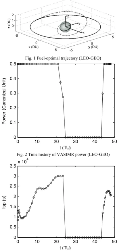
[image:4.595.317.521.264.704.2]The total flight time is 48.1613TU, which is about 12 hours. The terminal mass percent is 96.51% and the consumed fuel is 3.49%. Fig.1 is the flight trajectory. Fig.2 is time history of VASIMR power, namely, switching structure. It is obvious that Gauss Pseudo method clearly catched the switching structure which is “On-Off-On”.
Fig. 1 Fuel-optimal trajectory (LEO-GEO)
0 10 20 30 40 50
0 0.1 0.2 0.3 0.4 0.5
t (TU)
P
ow
er
(
C
anoni
cal
U
ni
t)
Fig. 2 Time history of VASIMR power (LEO-GEO)
0 10 20 30 40 50
0 0.5 1 1.5 2 2.5 3 3.5x 10
4
t (TU)
Is
p (
s)
inclination which reached the terminal boundary conditions precisely.
0 10 20 30 40 50
0 2 4 6 8
a (
D
U
)
0 10 20 30 40 50
0 0.2 0.4
e
0 10 20 30 40 50
0 10 20 30
i (
D
eg)
[image:5.595.327.520.99.252.2]t (TU)
Fig. 4 Time history of a, e, i (LEO-GEO)
B. LEO-Sun Synchronous Orbit (SSO)Transfer
This example demonstrates the ability of VASIMR engine to large inclination change transfer. The inclination changes from 28.5° to 99.5°. Initial orbit elements is given as: a0=6878km,
0
e =0.001, i0=28.5°, Ω =0 10°, ω0=10°, υ0=0°. Terminal
orbit elements: af = 7378km, ef = 0.001, if = 99.5°, f
Ω =20°, ωf =10°, υf is free.
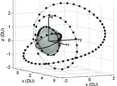
Again, Gauss Pseudospectral method shows its powerful ability in this example. This problem is firstly solved by using only 20 Gauss points. It is surprising that Gauss Pseudospectral catched the solution with so few Gauss points, although the solution is not smooth enough. The results with 20 Gauss Points are: total flight time is 78.0170TU which is about 19.6 hours; final mass ratio is 93.07%. The flight trajectory and time history of specific impulse with 20 Gauss points are shown in Fig.5 and Fig.6. They are not very smooth.
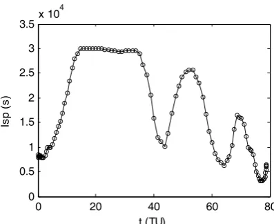
[image:5.595.322.521.101.414.2]Then, using the results from the first solution as initial guess, the same problem is refined using 100 Gauss points. The refined results with 100 Gauss points are: total flight time is 78.8320TU which is about 19.8 hours; final mass ratio is 93.40%. It is obvious that the results with 20 Gauss points and the results with 100 Gauss points are quite close. The flight trajectory, time history of specific impulse and orbital elements with 100 Gauss points are shown in Fig.7, Fig.8 and Fig.9, respectively. They are much smoother than the first results.
Fig. 5 Fuel-optimal trajectory (LEO-SSO, 20 Gauss points)
0 20 40 60 80
0 0.5 1 1.5 2 2.5 3 3.5x 10
4
t (TU)
Is
p (
s)
Fig. 6 Time history of VASIMR specific impulse (LEO-SSO, 20 Gauss points)
[image:5.595.63.265.110.417.2] [image:5.595.323.521.454.600.2]0 20 40 60 80 0
0.5 1 1.5 2 2.5 3 3.5x 10
4
t (TU)
Is
p (
[image:6.595.61.260.83.245.2]s)
Fig.8 Time history of VASIMR specific impulse (LEO-SSO, 100 Gauss points)
0 20 40 60 80
0 2 4 6
a (
DU)
0 20 40 60 80
0 0.5 1
e
0 20 40 60 80
0 50 100
i (
D
eg)
[image:6.595.320.520.202.728.2]t (TU)
Fig. 9 Time history of a, e, i (LEO-SSO, 100 Gauss points)
C. LEO-Molniya Transfer
A Molniya orbit is a representative elliptic inclined orbit. This example demonstrates the VASIMR engine ability of transferring to general inclined elliptic orbit. And it also shows the ability of Gauss Pseudospectral to deal with complicated trajectory optimization.
Initial orbit elements: a0=6878km, e0=0.001, i0=28.5°, 0
Ω = 10°, ω0= 10°, υ0= 0°. Terminal orbit elements:
f
a =26565km, ef =0.7355, if =63.4°, Ω =f 20°, ωf =270°, f
υ is free.
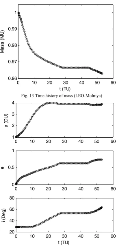
In this example, 100 Gauss points are used to obtain the solutions. The total flight time is 53.2192TU, which is about
13.4 hours. Terminal mass is 96.29% and the consumed fuel is 3.71%.
Fig.10 is the fuel-optimal flight trajectory with VASIMR engine. Fig.11 is time history of VASIMR power. Just like the last example, the VASIMR engine switching structure is catched properly by Gauss Pseudospectral again, which is “On-Off-On”. Fig.12 is the time history of specific impulse. Fig.13 is time history of mass. And Fig.14 is the time history of a, e, i during the transfer from LEO to Molniya orbit which also satisfied the terminal conditions.
Fig. 10 Fuel-optimal trajectory (LEO-Molniya)
0 10 20 30 40 50 60
0 0.1 0.2 0.3 0.4 0.5
t (TU)
P
ow
er
(
C
anoni
cal
U
ni
t)
Fig. 11 Time history of VASIMR power (LEO-Molniya)
0 10 20 30 40 50 60
0 0.5 1 1.5 2 2.5 3 3.5x 10
4
t (TU)
Is
p (
s)
[image:6.595.64.263.288.581.2]0 10 20 30 40 50 60 0.96
0.97 0.98 0.99 1
t (TU)
M
ass (
M
U
)
Fig. 13 Time history of mass (LEO-Molniya)
0 10 20 30 40 50 60
1 2 3 4
a (
DU)
0 10 20 30 40 50 60
0 0.5 1
e
0 10 20 30 40 50 60
20 40 60 80
i (
D
eg)
[image:7.595.61.264.89.518.2]t (TU)
Fig. 14 Time history of a, e, i (LEO-Molniya) V. CONCLUSION
Trajectory optimization problem with variable specific impulse magnetoplasma rocket (VASIMR) engine is studied using a newly developed method called Gauss Pseudospectral method. Three representative trajectory optimization problems are solved, which consist of an orbit raising problem, a large inclination change problem and a general inclined elliptic orbit transfer problem. These results show that: 1) VASIMR engine can be applied to different kind of orbital transfer problems. Because of the large regulable specific impulse, VASIMR engine can greatly increase the payload ratio and it is suitable for future big payload flight mission. 2) Gauss Pseudospectral method is a powerful method for complex trajectory optimization problems. The results in this paper show its ability to deal with different kind of trajectory optimization problems. Especially, it can catch the switching structure properly for the problems whose switching structure is unknown without solving the difficult TPBVP. A large mount of numerical
studies have been done by the author. It shows that it is much easier and faster to find the solutions using Gauss Pseudospectral method than using classical Pontryagin’s minimum principle (Benson has proved the optimality conditions from Gauss Pseudospectral method is equivalent to the discretized form of the first-order necessary conditions of the optimal control problem).
REFERENCES
[1] C. A. Kluever, “Geostationary orbit transfers using solar electric propulsion with specific impulse modulation,” Journal of Spacecraft and Rockets, Vol. 41, No. 3, 2004, pp. 461-466.
[2] Sang-Young Park, Kyu-Hong Choi, “Optimal low-thrust intercept/rendezvous trajectories to earth-cross objects,” Journal of
Guidance, Control and Dynamics, Vol. 28, No. 5, 2005, pp. 1049-1055.
[3] Juan Senent, Cesar Ocampo, Antonio Capella, “Low-thrust variable-specific-impulse transfers and guidance to unstable periodic orbits,” Journal of Guidance, Control, and Dynamics, Vol.28, No. 2, 2005, pp. 280-290.
[4] Hans Seywald, Carlos M Roithmayr, Troutman Patrick A Troutman and Sang-Young Park, “Fuel-optimal transfers between coplanar circular orbits using variable-specific-impulse engines,” Journal of Guidance,
Control, and Dynamics, Vol. 28, No. 4, 2005, pp. 795-800.
[5] J. T. Betts, “Survey of numerical methods for trajectory optimization,”
Journal of Guidance, Control, and Dynamics, Vol. 21, No. 2, 1998, pp.
193–207.
[6] D. A. Benson, G. T. Huntington, T. P. Thorvaldsen, A. V. Rao, “Direct trajectory optimization and costate estimation via an orthogonal collocation method,” Journal of Guidance, Control, and Dynamics, Vol. 29, No. 6, 2006, pp. 1435–1440.
[7] G. T. Huntington, D. A. Benson, and A. V. Rao, “Post-optimality evaluation and analysis of a formation flying problem via a Gauss Pseudospectral Method,” AAS Paper 05-339, 2005.
[8] G. T. Huntington, A. V. Rao, “Optimal spacecraft formation configuration using a Gauss Pseudospectral Method,” AAS Paper 05-103, 2005.