Genetic Algorithm Optimized PI and Fuzzy Sliding Mode Speed Control for DTC Drives

(1)

Genetic Algorithm Optimized PI and Fuzzy

Sliding Mode Speed Control for DTC Drives

Shady M. Gadoue, D. Giaouris, and J.W. Finch

Abstract— This paper presents a detailed comparison between a conventional PI controller and a variable structure controller based on a fuzzy sliding mode strategy used for speed control in direct torque control induction motor drive. Genetic algorithms are used to tune the PI controller gains to ensure optimal performance. The performance of the two controllers are investigated and compared for different dynamic operating conditions such as of reference speed and for load torque step changes at nominal parameters and in the presence of parameter variation and imprecision. Results show that the PI controller has better performance for nominal operating conditions while the fuzzy sliding mode is more robust against parameter variation and uncertainty, and is less sensitive to external load torque disturbances with a fast dynamic response.

Index Terms—Direct Torque Control, Fuzzy Logic, Genetic Algorithms, Induction motor, Sliding mode control

I. INTRODUCTION

Design of the speed controller greatly affects the performance of an electric drive. PI speed controllers are widely used in industrial applications due to their simple structure. However, because of the continuous variation of machine parameters, model uncertainties, nonlinear dynamics and system external disturbances, fixed-gain PI controllers may become unable to provide the required control performance [1], [2]. Therefore, continuous adaptation of the controller parameters becomes desirable when high performance is required from the drive system [1], [3]. Genetic Algorithms (GA) are adaptive search techniques based on a “survival of the fittest” biological concept. They can yield an efficient and effective way for optimization applications by searching for a global minimum without needing the derivative of a cost function [4], [7]. Therefore, GA can be applied in tuning the gains of PI controller to ensure optimal control performance at nominal operating conditions. However, another solution to the problem is to entirely replace the PI controller by adaptive control structures such as Model Reference Adaptive Control (MRAC), Sliding Mode Control (SMC), self tuning and Artificial Intelligence schemes [1]. The majority of these

designs have been successfully applied to vector control induction motor drives.

Manuscript received March 22, 2007.

This work was supported by The Ministry of Higher Education, Arab Republic of Egypt.

The authors are with the School of Electrical, Electronic and Computer Engineering, Newcastle University, Newcastle upon Tyne, NE1 7RU, UK.

Corresponding author: Shady Gadoue (phone +44-(0)191-222-7588; fax: +44-(0)191-222-8180; e-mail: [email protected]).

(other e-mails: [email protected], [email protected]).

Among these different proposed designs, the sliding mode control strategy has shown robustness against motor parameter uncertainties and unmodelled dynamics, insensitivity to external load disturbance, stability and a fast dynamic response [2], [4], [5]. Hence it is found to be very effective in controlling electric drives systems. Large torque chattering at steady state may be considered as the main drawback for such a control scheme [2]. One way to improve sliding mode controller performance is to combine it with Fuzzy Logic (FL) to form a Fuzzy Sliding Mode (FSM) controller [6].

The purpose of this paper is to provide a comprehensive analysis and detailed comparison between a FSM speed controller and a GA optimized PI controller in terms of robustness, disturbance rejection capability, sensitivity to stator resistance variation and uncertainty in motor inertia. The comparison is carried out based on assigning a performance index in terms of speed error to provide a numerical comparison of their performances when applied to a Direct Torque Control (DTC) induction motor drive. A modified sliding mode control law is derived based on Lyapunov theory for the electromagnetic torque demand to ensure system stability. The effectiveness of this control strategy is demonstrated through tests at different dynamic operating conditions.

This paper is organized as follows. In section II, the DTC strategy for induction motor control is described. Section III describes how GA can be applied in tuning the PI controller gains. In section IV, the detailed derivation of the sliding mode speed control law based on Lyapunov theory is presented. In section V, simulation results are presented. Conclusions are then summarized in the last section.

II. DTCSTRATEGY

(2)

[image:2.612.335.490.226.481.2] [image:2.612.53.297.243.391.2]

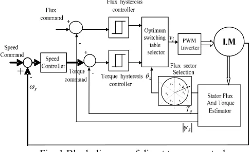
In principle, DTC is a direct hysteresis stator flux and electromagnetic torque control which triggers one of the eight available discrete space voltage vectors generated by a Voltage Source Inverter (VSI) in order to keep stator flux and motor torque within the limits of two hysteresis bands [3]. The correct application of this principle allows a decoupled control of flux and torque. Basically, the status of the errors of stator flux magnitude |ψs| and electromechanical torque Te are detected and digitalized by simple two- and three-level hysteresis comparators. An optimum switching table is then used to determine the status of three switches S1, S2, S3 and the corresponding voltage space vector vi depending on the stator flux region (θs). The stator flux position (θs) is determined by dividing the d-q plane into six 600_{regions. Simple three sign}

detectors are used to determine the sector where the stator flux exists.

s

ψ

e T s

θ i v

r ω

Fig. 1 Block diagram of direct torque control The primary space voltage vector of the PWM inverter vs

can be expressed in terms of the inverter switching states S1, S2,

S3 and the DC link voltage Vas:

(

)

⎥

⎦ ⎤ ⎢

⎣ ⎡

⎭ ⎬ ⎫ ⎩ ⎨ ⎧ + ⎭ ⎬ ⎫ ⎩ ⎨ ⎧ + = + =

3 4 exp 3

2 exp 3

2 ,

, ₂ ₃ ₁ ₂ ₃

1S S vsd jv V S S j π S j π

S _sq

s

v (1)

where vsd and vsq are the d-axis and q-axis stator voltage components in the stationary reference frame.

The stator flux and the electromagnetic torque can be represented by [3]:

(

v_sd R_si_sd dt

sd =

∫

−

ψ

)

(2)

(

v_sq R_si_sq

)

dt

sq =

∫

−

ψ (3)

(

sd sq sq sd

e P i i

T = ψ −ψ

2

3

)

₍₄₎

where isd, isq, ψsd and ψsq are the d-axis and q-axis stator current and flux linkage components in the stationary reference frame.

If the drive contains a speed control loop, then the reference speed input is compared with the actual motor speed and the speed error is fed to a speed controller. The output of the speed controller is the reference electromagnetic toque.

III. GENETIC ALGORITHMS

GA is a stochastic global adaptive search optimization technique based on the mechanisms of natural selection. Recently, GA has been recognized as an effective and efficient technique to solve optimization problems. Compared with other optimization techniques, such as simulating annealing

and random search method techniques, GA is superior in avoiding local minima which is a common aspect of nonlinear systems. Furthermore, GA is a derivative-free optimization technique which makes it more attractive for applications that involve non smooth or noisy signals. GA starts with an initial population containing a number of chromosomes where each one represents a solution of the problem which performance is evaluated by a fitness function. Basically, GA consists of three main stages: Selection, Crossover and Mutation. The application of these three basic operations allows the creation of new individuals which may be better than their parents. This algorithm is repeated for many generations and finally stops when reaching individuals that represent the optimum solution to the problem [4], [7]. The GA architecture is shown in Fig.2.

Fig. 2 Genetic Algorithm Architecture

Due to its effectiveness in searching nonlinear, multi-dimensional search spaces, GA can be applied to the tuning of PI speed controller gains to ensure optimal control performance at nominal operating conditions. The genetic algorithm parameters chosen for the tuning purpose are shown in Table I.

Table I

Genetic algorithm parameters

GA property Value/ Method GA property Value/ Method

Number of

generations 10

Selection method

Stochastic Universal Selection (SUS) No of

chromosomes in each generation

8 Crossover _method Double-point

No of genes in each chromosome

2 Crossover _probability 0.7

Chromosome

(3)

The cost function used to evaluate the individuals of each generation can be chosen to be the Integral Time of Absolute Error (ITAE). The mathematical expression of this cost function can be written as:

( )

t dt e t ITAE

t

∫ =

0

(5) During the search process GA looks for the optimal setting of the PI speed controller gains which minimizes the cost function (ITAE). This function is considered as the GA's evolution criterion which has the advantage of avoiding cancellation of positive and negative errors. Each chromosome represents a solution of the problem and hence it consists of two genes: the first one is the Kp value and the other one is the Ki value: so the chromosome vector is [Kp Ki] where the range of each gain must be specified.

IV. FUZZY SLIDING MODE CONTROLLER

SMC is considered as an effective and robust control strategy. It is mainly a Variable Structure Control (VSC) with high frequency discontinuous control action which switches between several functions depending on the system states. This forces the states of the system to slide on a predefined hypersurface. The plant states are mapped into a control surface using different continuous functions and the discontinuous control action switches between these several functions according to plant state value at each instant to achieve the desired trajectory. SMC is known for its capability to cope with bounded disturbance as well as model imprecision which makes it ideal for the robust nonlinear control of induction motor drives [8], [9]. To design a sliding mode speed controller for the induction motor DTC drive, consider the mechanical equation:

e L T

T P B P

J_ω₊ _ω₊ ₌

& (6) where ω is the rotor speed in electrical rad/s, rearranging to get:

ω ω

J B T J P T J P

L e− −

=

& (7) Considering ∆a and ∆b as bounded uncertainties introduced by system parameters J and B, (7) can be rewritten as [10]:

(

a+∆a

) (

+ b+∆b

)

Te+cTL

= ω

ω& (8)

where:

J

P

c

J

P

b

J

B

a

=

−

;

=

;

=

−

Defining the state variable of the speed error as:

( ) ( )

t t

( )

t

e =ω −ω* (9) Combining (8) with (9) and taking the derivative of (9) yields:

( )

t ae

( )

t b

{

T

( ) ( )

t dt

}

e_& = + _e + (10) where d(t) is the lumped uncertainty defined as:

( )

e TL

b c T b

b t b

a t

d =∆ ω +∆ + (11) and

( )

_ω*

b a t T t

Te = e + (12)

Defining a switching surface s(t) from the nominal values of system parameters a and b [5], [10]:

( ) ( ) (

t =et −_∫t a+bk

) ( )

e d s

0

τ

τ (13) Such that the error dynamics at the sliding surfaces

( ) ( )

t =s&t =0

will be forced to exponentially decay to zero, then the error dynamics can be described by:

( ) (

t a bk

) ( )

et

e& = + (14) where k is a linear negative feedback gain [10].

A speed control law can be defined as:

( )

t

( )

s

( )

t ke

T_e = −βsgn (15) where β is known as hitting control gain used to make the sliding mode condition possible and the sign function can be defined as [6]:

( )

⎪ ⎭ ⎪ ⎬ ⎫

⎪ ⎩ ⎪ ⎨ ⎧

< −

= > =

0 1

0 0

0 1

sgn

s if

s (16)

The final electromagnetic torque command Te* of the output of the sliding mode speed controller can be obtained by directly substituting (15) into (12).

Basically, the control law for Te* is divided into two parts: equivalent control ueq which defines the control action when the system is on the sliding mode and switching part us which ensures the existence condition of the sliding mode. If the friction B is neglected, expressions for ueq and us can be written as:

( )

t u

( )

s

( )

t ke

u_eq = ; _s =−βsgn (17) To guarantee the existence of the switching surface consider a Lyapunov function [6]:

( )

t s

( )

t

v 2

2 1

= (18) Based on Lyapunov theory, if the functionv&

( )

t is negative definite, this will ensure that the system trajectory will be driven and attracted toward the sliding surface s(t) and once reached, it will remain sliding on it until the origin is reached asymptotically [6]. Taking the derivative of (18) and substituting from the derivative of (13):

( ) ( ) ( )

( ) ( ) (

⋅

{

− +

) ( )

≤0

=

}

⋅ =

t e bk a t e t s

t s t s t v

& &

& ₍₁₉₎

Substitute from (10) into (19):

( ) ( ) ( )

t st st

{

bT

( )

t bd

( )

t bke

( )

t

}

s ⋅& = ⋅ _e + − (20) Using (15), gives:

( ) ( ) ( )

t ⋅st =st ⋅

{

−b

(

sgn

( ) ( )

s −d t

)

}

≤0

(4)

To ensure that (21) will be always negative definite, the value of the hitting control gain β should be designed as the upper bound of the lumped uncertainties d(t), i.e.

( )

t d ≥

β (22) However, it is difficult practically to estimate the bound of uncertainties in (11). Therefore the hitting control gain βhas to be chosen large enough to overcome the effect of any external disturbance [5], [6]. Therefore the speed control law defined in (15) will guarantee the existence of the switching surface s(t) in (13) and when the error function e(t) reaches the sliding surface, the system dynamics will be governed by (14) which is always stable [10]. Moreover, the control system will be insensitive to the uncertainties ∆a , ∆b and the load disturbance

TL [10].

The use of the sign function in the sliding mode control (15) will cause high frequency chattering due to the discontinuous control action which represents a severe problem when the system state is close to the sliding surface [6]. To overcome this problem a boundary layer Φ is introduced around the switching surface and the sign function (16) will be replaced by a saturation function sat(s /Φ) [6]. The choice of Φ is crucial; small values of Φ may not solve the chattering problem and large values may increase the steady state error [6], requiring a compromise choice when selecting the boundary layer thickness.

Another approach to reduce the chattering phenomenon is to combine FL with a SMC [6]. Hence a new Fuzzy Sliding Mode (FSM) controller is formed with the robustness of SMC and the smoothness of FL. The switching functions of sliding mode and FSM schemes are shown in Fig. 3. In this technique the saturation function is replaced by a fuzzy inference system to smooth the control action. The block diagram of the hybrid fuzzy sliding mode controller is shown in Fig. 4.

[image:4.612.332.549.243.433.2]

(a) (b)

Fig. 3 Switching functions (a) Sliding mode (b) Fuzzy sliding mode

The If-Then rules of the fuzzy logic controller can be written as [6]:

If s is BN then us is BIGGER If s is MN then us is BIG If s is JZ then us is MEDIUM If s is MP then us is SMALL If s is BP then us is SMALLER

V. SIMULATION RESULTS AND DISCUSSION

To compare the two speed controller design strategies, PI-GA and FSM, a DTC of a 7.5 kW squirrel cage induction motor shown in Fig. 1 is simulated using Matlab-Simulink software. The parameters of each controller are:

PI-GA: Using the GA parameters given in Table I, the optimal

PI controller gains at 50 rad/s electric speed command and 25% rated torque applied to the motor during the tuning process are found to be Kp= 127, Ki= 4.

FSM: The controller coefficients used in the simulation are: k

=-2.3e-4, β = 100. The membership functions for the input and output of the FL controller are obtained by trial error to ensure optimal performance and are shown in Fig.5.

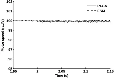
[image:4.612.57.288.445.570.2]

To examine the disturbance rejection capability of both schemes, a step change in the load torque from 25% to 75% of its rated value is applied at t=2s when the motor is running at 100 rad/s. When the load torque change is applied, PI-GA shows a poor disturbance rejection capability with a steady state error of 0.13% while FSM exhibits insensitivity to sudden load change. The response of the two schemes is shown in Fig.6.

Fig. 4 Fuzzy sliding mode speed controller

(a) (b)

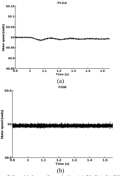
Fig. 5 Fuzzy logic membership functions (a) input (b) output To study the effect of electric parameter variation on the performance of both controllers, the drive is run with a 50 rad/s speed command, 25% rated torque and nominal machine parameters, at t=1s a 50% step increase in the motor stator resistance Rs is applied. The sensitivity of stator resistance is investigated because its variation greatly affects the performance of the DTC drive. The response of the two schemes is shown in Fig.7 where PI-GA shows oscillations with a negligible steady state error while FSM proves less sensitivity to Rs variation. However, the steady state speed obtained from FSM has more ripples around the command speed 50 rad/s.

1.95 2 2.05 2.1 2.15

95 96 97 98 99 100 101 102

Time (s)

M

o

to

r s

p

eed

(

rad/

s

)

PI-GA FSM

[image:4.612.343.532.602.728.2]

(5)

0.9 1 1.1 1.2 1.3 1.4 1.5 49.85

49.9 49.95 50 50.05 50.1 50.15

Time (s)

M

o

to

r speed

(

rad/

s

)

PI-GA

(a)

0.9 1 1.1 1.2 1.3 1.4 1.5 49.5

50 50.5

Time (s)

M

o

to

r speed

(

rad

/s

)

FSM

[image:5.612.76.268.50.332.2]

(b)

Fig. 7 Sensitivity to Rs variation (a) PI-GA (b) FSM Figure 8 shows the speed response obtained from both schemes with uncertainty in the motor inertia J. The nominal value of J is used in the FSM controller. It is clear that the steady state error in the motor speed increases as the percentage uncertainty increases in PI-GA scheme. The steady state error with 100% uncertainty is 0.14%. By contrast the FSM scheme is insensitive to motor inertia uncertainty due to the proper choice of β in (22).

0 0.1 0.2 0.3 0.4 0.5

47 47.5 48 48.5 49 49.5 50 50.5 51

PI-GA

Time (s)

M

o

tor sp

eed

(

rad

/s)

J 0.5J 1.5J 2J

(a)

0 0.1 0.2 0.3 0.4 0.5

47 47.5 48 48.5 49 49.5 50 50.5 51

FSM

Time (s)

M

o

tor sp

eed

(

rad

/s

)

J 0.5J 1.5J 2J

[image:5.612.337.549.282.722.2]

(b)

Fig. 8 Speed responses with J uncertainty (a) PI-GA (b) FSM

To study the drive performance with a change in the command speed with nominal and uncertain parameters, a speed reference step change from 50 rad/s to 200 rad/s at 25% rated load and nominal parameters is applied to the drive at t=1s. The response of both schemes is shown in Fig. 9. FSM shows faster response and the motor speed reaches the command in 0.125s with a negligible steady state error while the PI-GA scheme shows slower response (0.16s) with 0.175% steady state error. The switching function s(t) in (13) is shown in Fig. 10. When the speed command changes, the speed error initially drops to a big negative value and as long as (21) is negative definite, it will be attracted to the sliding surface s=0 and when reaches it, the error dynamics will slide on this switching surface.

Another test is performed by applying a speed reversal command from 50 rad/s to -50 rad/s at 25% rated load with 50% uncertainty in motor inertia J. As shown in Fig. 11, FSM still shows faster dynamics and reaches the command speed in 0.1s with negligible steady state error compared with 0.18s and 0.44% steady state error for PI-GA scheme.

1.1 1.15 1.2 1.25 1.3

190 195 200 205

Time (s)

M

o

to

r sp

ee

d

(

rad

/s

)

PI-GA FSM

Fig. 9 Speed Response with step change in speed demand

0 0.5 1 1.5 2

-160 -140 -120 -100 -80 -60 -40 -20 0 20

FSM

Time (s)

s(

t)

Fig. 10 Switching surface of FSM scheme

0.9 1 1.1 1.2 1.3 1.4 1.5 -50

0 50

Time (s)

M

o

to

r spee

d (

rad/

s

)

PI-GA FSM

[image:5.612.77.263.449.722.2]

(6)

[image:6.612.49.282.205.671.2]

During normal operating conditions when the drive is running at 50 rad/s speed command, 25% rated torque and nominal machine parameters, PI-GA shows less ITAE compared to FSM since it uses the optimal controller gains for normal operating conditions. However, if the drive runs at a speed command of 100 rad/s at nominal parameters and 25% rated load, the speed response obtained from PI-GA scheme shows higher ITAE with 0.2% steady state error compared with a negligible one from FSM scheme. This is because the PI gains are optimized at 50 rad/s. The simulation results are summarized in Table II.

Table II

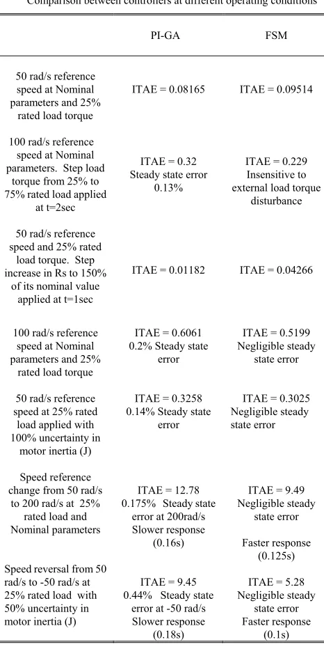
Comparison between controllers at different operating conditions

VI. CONCLUSION

In this paper a detailed comparison between GA optimized PI and FSM speed controllers is presented. A modified control law for the electromagnetic torque command is derived for DTC drive based on Lyapunov theory for FSM control. PI-GA shows better performance at nominal operating conditions while FSM proves robustness against stator resistance variation, uncertainty in motor inertia and insensitivity to load torque disturbance as well as faster dynamics with negligible steady state error at all dynamic operating conditions.

APPENDIX

MOTOR PARAMETERS

PI-GA FSM

50 rad/s reference speed at Nominal parameters and 25%

rated load torque

ITAE = 0.08165 ITAE = 0.09514

100 rad/s reference speed at Nominal parameters. Step load

torque from 25% to 75% rated load applied

at t=2sec

ITAE = 0.32 Steady state error

0.13%

ITAE = 0.229 Insensitive to external load torque

disturbance

50 rad/s reference speed and 25% rated

load torque. Step increase in Rs to 150%

of its nominal value applied at t=1sec

ITAE = 0.01182 ITAE = 0.04266

100 rad/s reference speed at Nominal parameters and 25%

rated load torque

ITAE = 0.6061 0.2% Steady state

error

ITAE = 0.5199 Negligible steady

state error

50 rad/s reference speed at 25% rated

load applied with 100% uncertainty in

motor inertia (J)

error

ITAE = 0.3025 Negligible steady state error

Speed reference change from 50 rad/s

to 200 rad/s at 25% rated load and Nominal parameters

error at 200rad/s Slower response

(0.16s)

state error

Faster response (0.125s) Speed reversal from 50

rad/s to -50 rad/s at 25% rated load with 50% uncertainty in motor inertia (J)

error at -50 rad/s Slower response

(0.18s)

state error Faster response

(0.1s)

7.5 kW, 3-phase, 220V, 60 Hz, P = 4, Rs = 0.15 Ω, Rr = 0.17 Ω,

Ls = 0.035 H, Lr = 0.035 H, Lm = 0.0338 H, J = 0.14 Kg. m2

REFERENCES

[1] M. N. Uddin, T. S. Radwan, M. Rahman, “Performance of fuzzy-logic-based indirect vector control for induction motor drive,” IEEE Trans. Ind. Applicat.,

Vol.38, No. 5, Sept./Oct. 2002, pp. 1219-1225.

[2] F. Barrero, A. Gonzalez, A,. Torralba, E. Galvan and L. G.Franquelo, “Speed control of Induction Motors using a novel Fuzzy Sliding Mode structure,”

IEEE Trans. Fuzzy Syst., Vol.10, No.3, June 2002, pp. 375-383.

[3] Y. Lai and J. Lin, “New hybrid Fuzzy controller for Direct Torque Control Induction Motor drives,” IEEE Trans. Power Electron., Vol. 18, No. 5, Sept. 2003, pp. 1211-1219

[4] F. Lin, W. Chou and P. Huang, “Adaptive sliding mode controller based on real time genetic algorithm for induction motor servo drive,” IEE Proc. Electr. Power Appl., Vol.150, No.1, Jan.2003, pp. 1-13.

[5] O. Barambones, A.J. Garrido, F.J. Maseda and P. Alkorta, “An adaptive sliding mode control law for Induction Motor Using field oriented control theory,” Proc. IEEE International Conf. on Control Applications, 2006, pp. 1008-1013.

[6] J. Lo and Y. Kuo, “Decoupled Fuzzy Sliding Mode Control,” IEEE Trans. Fuzzy Syst., Vol.6, No. 3, Aug. 1998, pp. 426-435.

[7] P.Vas, Artificial-Intelligence-Based Electrical Machines and Drives-Application of Fuzzy, Neural, Fuzzy-Neural and Genetic Algorithm Based Techniques. New York: Oxford University Press, 1999.

[8] V. I. Utkin, “Sliding Mode control design principles and applications to electric drives,” IEEE Trans. Ind. Electron., Vol. 40, No. 1, Feb. 1993, pp. 23-36.

[9] W. S. Levine (Ed.), The control handbook, CRC Press, 1996.

[10] K. Shyu and H. Shieh, “A new switching surface sliding mode speed control for induction motor drive systems,” IEEE Trans. Power Electron.,