A Multistage Approach to the Design of Prototype
Filters for Modulated Filter Banks
Neela R. Rayavarapu(Member IEEE) and Neelam Rup Prakash(Member IEEE)
Abstract: When filter banks are used in multicarrier
modulation the transition bandwidth of the filter is usually very narrow. This is because the bandwidth of the filters is determined by the number of subchannels and the greater the number of channels lesser will be the transition bandwidth. The order of the filter being inversely proportional to the transition bandwidth is generally very high. Hence computational complexity is also very high. We propose a method that will help reduce this complexity by designing the decimators/interpolators in the subchannels using a multistage approach. We compare the saving obtained in comparison to direct design approaches. We will also compare the performance of a cosine modulated filter bank designed in this way with direct design methods.
Keywords: decimator, interpolator, multicarrier modulation,
multistage, transition bandwidth,
1. Introduction
Digital Subscriber Line (xDSL) applications use a multicarrier modulation technique called as Discrete Multitone (DMT) for the purpose of high bit rate transmission over the commonly used twisted pair copper wires. This eliminates bottlenecks in the data access network between the central office and the end user. This has been made possible by the use of, amongst other things , advanced signal processing technology. One such area of signal processing, filter banks , has found vast applications is several areas of digital communication , such as high speed DSL services for internet [1][2].
In Fig.1 is shown the block diagram of a multicarrier modulation system that uses multirate filter banks . The modulation and demodulation is performed using filters and fast transforms such as
Manuscript submitted on February 15, 2010.
Ms. Neela Rayavarapu is with the Department of Electronics and Communication Engineering, Chitkara Institute of Engineering and Technology, Rajpura, Punjab, India. (email:
neela.rayavarapu@chitkara.edu.in)
Dr. Neelam Rup Prakash is with the Department of Electronics and Communication Engineering, Punjab Engineering College, Chandigarh. India.
FFT and DCT. The multirate filter bank is composed of the synthesis and the analysis filter banks that are used for performing modulation and demodulation.
Each channel of the synthesis filter bank consists of an upsampler cascaded with a filter, together called as the interpolator, and the analysis filter bank consists of a filter followed by a downsampler together termed as a decimator.
The up sampling and the down sampling factors will be determined by the number of subchannels of the system and greater the number of channels greater will be upsampling/downsampling factor and smaller will be the transition bandwidth. This will obviously lead to longer length filters being used. This will in turn increase the computational complexity involved in the implementation of the decimators and the interpolators.
In order to minimize computation a multistage approach to the decimator and interpolator shown in Fig2. and Fig 3. is used. This is based on the IFIR approach suggested by Neuvo et al [3]. We will briefly explain this method and see how it may used to obtain multistage implementations.
S/P convertor
and encoder
Modulat or
P/S Convertor
Chan
nel
S/P Convertor Demodulat
or equalizer
De
co
de
r
,P/S conver
to
r
o/p i/p
2. IFIR filter
(a)
(b)
(c)
(d)
Fig 4. Stages of the IFIR filter.
Say the desired filter designed according to certain set specifications has order N and a transition bandwidth of Δf. If this filter is stretched 2 fold then the transition band will be 2 Δf and the order of the stretched filter G(z) as shown in Fig.4(b) will be N/2. The frequency response of G(z2) is as
shown in (c). It has two pass bands, one the desired passband
and the other is its image centered on 2π/L where L is the
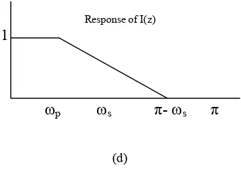
stretch factor, in this case 2. This image is to be suppressed by cascading the filter G(z2) with an image suppressor filter
I(z) as shown in (d), to obtain the desired response. The order of I(z) is very small as it has a very large transition band. The order of G(z) (model filter) will be a little more than N/2. Therefore since the order of the two filters is low the amount of computational complexity involved in implementing the filter is greatly reduced.
Fig. 5 IFIR filter for stretch factor L
3. Multistage Design
Consider the analysis filter bank in the figure shown below. For number of subchannels M that is large the analysis filter H(z) will be narrowband and may designed using the IFIR approach.
Response of I(z)
1
ω
pω
sπ- ω
sπ
[image:2.595.54.241.85.720.2]H(z)
M
Fig. 2. Decimation Decimator Filter
x(n) y(n)
[image:2.595.329.504.101.225.2]M
H(z)
Fig. 3. Up Sampler Interpolation Filter
x(n) y(n)
I(z)
G(zL)y(n) x(n)
Desired Narrow Band Response
1 H(z)
ω
pω
sπ
1
Stretched filter G(z)2ω
p2ω
sπ
Response of G(z2)
1
Desired undesiredLet us take the stretch factor M1 to be a factor of the
decimation factor M. Then we may represent the decimator structure in each channel as a cascade of the image suppressor
filter then down sampling by M1, the model filter G(z) and
then down sampling by M2 as shown in Fig. 5 below.
The computational complexity involved in the implementation of the filters is dependent on the order of the filter and the order of the Model filter G(z), Ng and the Image
suppressor filter I(z), Ni can be obtained from the equations
below.
Ng =
1 * 2 / ) ( 6 . 14 13 2 1 5 . 0 log 20 M p
s
(1)
Ni =
2 / ] ) ( 2 [ 6 . 14 13 5 . 0 log 20 1 2 1 M p s
(2)
The number of multiplications per unit time(MPU) is
Ng/M + Ni/M1 (3)
In the tables shown below the direct and multistage designs are compared on the basis of the filter order and the number of additions and multiplications involved in the implementation of the filter for different values of M and M1.
Note that M will remain fixed and M1 can take different
[image:3.595.63.260.89.233.2]values for given M
Table I: Variation of filter order with M.
Filter order
M Direct Design
IFIR Method
G(z) I(z) Total
8 M1=4 75 21 17 101
16 M1=8 150 21 32 200
M1=4 41 13 177
32 M1=16 298 21 64 400
M1=8 41 25 353
64 M1=32 596 21 129 801
M1=16 41 50 706
81 23 671 M1=8
From Table 1. the following inference can be drawn. As the value of M is increased the order of the conventional filter approximately doubles and the order of the model filter G(z) and of I(z) are significantly less. Also the order of G(z) and
I(z) is dependent on the value of the factor M1. As M1
[image:3.595.52.247.354.416.2]reduces the order of G(z) increases and that of I(z) reduces. Table 2. will show the effect of the multistage approach on the computation involved. The specifications we have chosen are δ1=.02, and δ2=.001. The passband and stop band
[image:3.595.303.534.411.756.2]edges have been chosen to be π/2M and π/M respectively.
Table II. Comparison on the basis of MPU
M Direct Design
IFIR Method
G(z) I(z) Total
8 M1=4 4.69 1.31 2.3 2.61
16 M1=8 4.69 .656 2 2.656
M1=4 2.56 1.63 4.19
32 M1=16 4.66 .328 2 2.328
M1=8 .641 1.56 2.2
64 M1=32 4.66 .164 2.02 2.184
M1=16 .32 1.56 1.88
.633 1.44 2.073 M1=8
[image:3.595.44.247.532.635.2]
Table III. Comparison on the basis of APU
M Direct Design
IFIR Method
G(z) I(z) Total
8 M1=4 9.38 2.63 4.25 6.88
16 M1=8 9.38 2.63 4 2.63
M1=4 2.56 3.25 5.81
32 M1=16 9.31 .656 4 4.656
M1=8 1.28 3.13 4.41
64 M1=32 9.31 .328 4.03 4.358
M1=16 .641 3.13 3.771
1.27 2.88 4.15 M1=8
H0(z)
H1(z)
HM-1(z)
x(n) x0(n)
x1(n)
xM-1(n)
Fig. 6 Analysis Filter Bank M
M
M
I(z) G(zM
1) M1M2
I(z) M1 G(z)
M2
What can be inferred from the Tables 2 and 3 is the following. The cost of implementation of the filter using direct design methods is almost independent of the number of subchannels. But the cost using multistage designs varies for different M. Also for a given M the computational cost is different for
different values of M1. This means therefore that there must
be some value of M1, where the computational cost is
minimum. We will now proceed to determine that value of M1
where the cost of implementation in terms of MPU is minimum for a fixed M.
Substituting (1) and (2) in (3) , differentiating the result with
respect to M1 and equating to zero we will get the value of
M1 that will obtain minimum MPU for a given value of M.
This is given by
M1(optimal) =
2 2 2 2 2 ) ( ) ( ) ( 2 ) ( ) ( 2 p s p s p s p s p s M M
M
(4)
Since the value of M1 we obtain from (4) may not exactly be a
factor of M we must choose an appropriate value that is close to it. On testing the values for different M1 and comparing, the
values that we have tabulated in Table (3) match very closely. So we may conclude that by factoring M suitably we can obtain maximum saving in computation cost. We have shown here, how the decimators of the analysis filter bank can be designed using the multistage approach. The interpolators in the case of the synthesis filter bank may also be designed using the multistage approach.
Next we will study that the characteristics of a prototype filter for a cosine modulated filter bank designed by this method and see how it compares with that of a filter obtained by direct design methods.
0 0.1 0.2 0.3 0.4 0.5 0.6 0.7 0.8 0.9 1
-250 -200 -150 -100 -50 0 50
magnitude response of G(z) and I(z)
normalised frequency /pi
m agn it ude i n d B G(z) I(z)
0 0.1 0.2 0.3 0.4 0.5 0.6 0.7 0.8 0.9 1 -150
-100 -50 0
50 magnitude response of the 32 channel filter bank
normalised frequency /pi
m agn it ud e i n dB
0.11 0.115 0.12 0.125 0.13 0.135 0.14 -5
0 5 10 15x 10
-3 amplitude distortion function
normalised frequency /pi
m a g n it ud e i n dB
Comparisons are obtained in the case of a 32 channel filter bank, using the method proposed by creusere and Mitra in [5] where the order of the filter by direct design is 511 where as for the same method using the multistage implementation the order of G(z) ia 69 and I(z) is 73 all specifications of the filters being the same for both methods.
We have chosen M1 to be 8 is is the factor closest to the
optimal value calculated using (4)
In the case of [5] the peak to peak amplitude distortion was marginally lower at .01
References
[1] Cherubini, G., Elfetheriou,E., Olcer,S., and Cioffi,J.M., “Filter bank modulation techniques Very high speed digital subscriber lines,” IEEE Communications Magazine, pp.98-104, May 2000.
[2] Nowrouzian,B., Wang,L., Agha, W., “An overview of discrete multitone modulation/demodulation systems in xDSL applications IEEE,2001
[3] Neuvo,Y., Dong,C.Y. and Mitra,S.K.,“Interpolated finite impulse response filters,” IEEE Trans. on Acoustics, Speech and Signal Processing, vol. ASSP-32, pp. 563-570, June 1984
[4] P.P Vaidyathan, Multirate Systems and Filter Banks. Prentice Hall, Englewood Cliffs, New Jersey, 1997. [5] Creusere, C.D. and Mitra. S.K., “ A simple method for
designing high quality prototype filters for M-channel Pseudo QMF banks, IEEE Trans. on Signal Processing, vol. 43, no.4, pp.1005-1007, April 1995.