Electric Motor Fault Diagnosis Based on Parameter Estimation Approach Using Genetic Algorithm

(1)

Electric Motor Fault Diagnosis Based on

Parameter Estimation Approach Using Genetic

Algorithm

Juggrapong Treetrong

Abstract— This paper proposes a new scheme of induction motor parameter estimation using Genetic algorithm (GA) for condition monitoring. The flux linkage model and torque model of an induction motor is adapted to the estimation. The scheme is developed to obtain all the motor parameters: stator and rotor resistance, stator and rotor leaking reactance and magnetizing reactance, which paves the way to diagnose different types of the faults. The scheme minimizes the difference between the measured and the predicted state variables: three phase currents and rotor speed. The scheme is evaluated firstly with different motor sizes and different load levels by simulation tests and then by the experimental data of the induction motors under normal operating condition at different load levels and fault conditions. The results from both tests show that the new scheme can estimate the parameters and predict the motor condition with sufficient accuracy for motor fault diagnosis.

Inedex terms— Induction Motor, Parameter Estimation, Genetic Algorithm, Condition Monitoring, Fault Detection

I. INTRODUCTION

Induction motors are the most widely used motors among different electric motors because of high level of reliability, efficiency and safety. Condition monitoring of induction motors can provide useful information so that the motor fault, if any, can be fixed at the earliest opportunity without affecting the plant requirement. Among many condition monitor methods such as vibration analysis, current signature processing, etc an online estimation of the motor parameters (stator and rotor resistance, stator and rotor reactance and magnetizing reactance) at a regular interval are the most potential approach to the diagnosis of the motor conditions with real engineering sense and real-time implementation. In addition, parameter estimation is the primary task for develop an automatic motor diver system. This means that the parameter estimation is important for both condition monitoring and control.

Conventionally, the parameter estimation is conducted by 3 classical tests: a locked-rotor test, a no-load test, and a DC test. However, these tests need special equipments and they are intrusive in nature and to be conducted under off-line condition. Thus, these tests may not always be feasible for the condition monitoring.

This work was sponsored by Department of Teacher Training in Mechanical Engineering, King Mongkut’s University of Technology North Bangkok, Pibul-Songklarm, Bangkok, 10800, Thailand, E-mail:

[email protected]

Considering the above limitations, a reliable and non-intrusive method is needed to estimate the motor parameters. Many such methods have been investigated over last several decades. Recursive Least-Square (RLS) has been applied to estimate motor parameters [1]-[3]. Treetong et al. [1] have used to estimate the stator related parameters using the RLS method. Horga et al. [2] have used the RLS method for the squirrel-cage induction motor related parameters. They used algorithm of the continuous parametric model of the induction motor. The model was based on a technique that used the Poisson moment functional theory. The RLS was also applied to determine the rotor resistance, self-inductance of the rotor winding, and the stator leakage inductance of a three-phase induction machine [3].

Extended Kalman Filter (EKF) is another optimisation technique used earlier to determine the motor parameters [4]-[5]. Velazquez et al. [4] have used the EKF method to identify the speed of an induction motor and rotor flux based on the measured quantities such as stator currents and DC link voltage. The model is performed at a synchronous rotating reference frame. In another study [5], the EKF is used to estimate speed of induction motor from speed-sensorless field-oriented control and direct-torque control of induction motors. The model can be estimated at a wide velocity range and persistent zero-speed operation.

(2)

Thus, this paper presents a model of the motor to estimate the motor parameters using the proposed GA method. The model is arranged from the flux linkage models and torque model of a squirrel-cage induction motor. The proposed GA method is used as a key algorithm to find the best parameter values. The fitness value is partly used to select the next generation of population. Simulation study is conducted with 3 different motor sizes and 5 different load levels of the induction motor. Having established the proposed method on the simulated examples, the method has then been applied to the experimental data of the two identical 3-phase induction motors under normal operating condition at different load. The results show that the proposed method can estimate the motor parameters effectively and indicate the motor condition with reliability

II. DYNAMIC MODEL OF INDUCTION MOTORS

The dynamic model employed in this paper is the Krause’s model [11]. It formulise the electromagnetic relation of the induction motor with a set of flux differential equations, rather than the voltage equations, which is used in most of the previous work for parameter estimation.. In particular, this model is adapted to the per-unit system and does not need to calculate inverse matrix. Therefore, it has fewer problems with numerical solution and can be more efficiently, compared with the current equations. The dynamic model written in magnetic flux linkage F in QD0 reference frame can be drived as

Eq.1-5, ⎥ ⎥ ⎦ ⎤ ⎢ ⎢ ⎣ ⎡ ⎟ ⎟ ⎠ ⎞ ⎜ ⎜ ⎝ ⎛ ⎟⎟ ⎠ ⎞ ⎜⎜ ⎝ ⎛ − + + − = qs ls ml qr lr ml ls s ds b e qs b qs F x x F x x x R F v dt dF 1 * * ω ω

ω (1)

⎥ ⎥ ⎦ ⎤ ⎢ ⎢ ⎣ ⎡ ⎟ ⎟ ⎠ ⎞ ⎜ ⎜ ⎝ ⎛ ⎟⎟ ⎠ ⎞ ⎜⎜ ⎝ ⎛ ₋ + + − = ds ls ml dr lr ml ls s qs b e qs b ds F x x F x x x R F v dt dF 1 * * ω ω

ω (2)

⎟⎟ ⎠ ⎞ ⎜⎜ ⎝ ⎛ − = s ls s s b s F x R v dt dF 0 0

0 _ω _* (3)

⎥ ⎥ ⎦ ⎤ ⎢ ⎢ ⎣ ⎡ ⎟ ⎟ ⎠ ⎞ ⎜ ⎜ ⎝ ⎛ ⎟⎟ ⎠ ⎞ ⎜⎜ ⎝ ⎛ − + + − − = qr lr ml qs lr ml lr r dr b r e qr b qr F x x F x x x R F v dt dF 1 * * ω ω ω

ω (4)

⎥ ⎥ ⎦ ⎤ ⎢ ⎢ ⎣ ⎡ ⎟ ⎟ ⎠ ⎞ ⎜ ⎜ ⎝ ⎛ ⎟⎟ ⎠ ⎞ ⎜⎜ ⎝ ⎛ − + + − − = _dr lr ml ds lr ml lr r qr b r e qr b dr _F x x F x x x R F v dt dF 1 * * ω ω ω

ω (5)

Where rotor speed is

ω

_r

(

e L

)

perunit r T T J p dt d − ⎟ ⎠ ⎞ ⎜ ⎝ ⎛ = 2 , ω (6)

The electric torque of the induction motor can be expressed by

(

ds qs qs ds

)

b

e F i F i

p

T ⎟ −

⎠ ⎞ ⎜ ⎝ ⎛ = ω 1 2 2

3 ₍₇₎

The base angular frequency

ω

_b

=

2 ×

π

×

50

and the motor parameters to be estimated:

R

s

,

R

r

,

x

m

,

x

ls and

lr

x

denoting stator resistance, rotor resistance, magnetizing reactance, stator leaking reactance and rotor leaking reactance respectively.

Eg. 1-6 are nonlinear differential equations. The solutions:

F

_qs,

F

_ds,

F

_qr,

F

_dr

F

₀_s,

ω

_r_,_perunit can be found easily through a fourth-order Runge-Kutta method. From the solutions of the model, the stator and rotor currents in DQ0 reference frame can be calculated

explicitly: ⎟ ⎟ ⎠ ⎞ ⎜ ⎜ ⎝ ⎛ ⎟⎟ ⎠ ⎞ ⎜⎜ ⎝ ⎛ + − ⎟⎟ ⎠ ⎞ ⎜⎜ ⎝ ⎛ = lr qr ls qs aq qs ls qs x F x F x F x

i 1 (8)

⎟ ⎟ ⎠ ⎞ ⎜ ⎜ ⎝ ⎛ ⎟⎟ ⎠ ⎞ ⎜⎜ ⎝ ⎛ + − ⎟⎟ ⎠ ⎞ ⎜⎜ ⎝ ⎛ = lr dr ls ds ad ds ls ds x F x F x F x

i 1 (9)

( s)

ls

s F

x

i0 0

1 ⎟⎟ ⎠ ⎞ ⎜⎜ ⎝ ⎛

= (10)

⎟ ⎟ ⎠ ⎞ ⎜ ⎜ ⎝ ⎛ ⎟⎟ ⎠ ⎞ ⎜⎜ ⎝ ⎛ + − ⎟⎟ ⎠ ⎞ ⎜⎜ ⎝ ⎛ = lr qr ls qs aq qr lr qr x F x F x F x

i 1 (11)

⎟ ⎟ ⎠ ⎞ ⎜ ⎜ ⎝ ⎛ ⎟⎟ ⎠ ⎞ ⎜⎜ ⎝ ⎛ + − ⎟⎟ ⎠ ⎞ ⎜⎜ ⎝ ⎛ = lr dr ls ds aq dr lr dr x F x F x F x

i 1 (12)

where * 1 1 1 1

− ⎟⎟ ⎠ ⎞ ⎜⎜ ⎝ ⎛ ₊ ₊ = lr ls m ml x x x x P b perunit r Sec rad r 2 , / , ω ω

ω = (13)

In order to calculate the fitness values in applying GA, variables in QD0:

i

qs,

i

dsand

i

s0 are transformed into 3

phase currents by a transformation matrix

K

_s

[

as bs cs

]

s s qd

abcs

i

K

i

=

₀

=

(14)

Where

i

_qd₀_s

=

[

i

_qs

i

_ds

i

_s₀

]

and

⎥ ⎥ ⎥ ⎦ ⎤ ⎢ ⎢ ⎢ ⎣ ⎡ + + − − = 1 )) 3 / 2 ( sin( )) 3 / 2 ( cos( 1 )) 3 / 2 ( sin( )) 3 / 2 ( cos( 1 ) sin( ) cos( π θ π θ π θ π θ θ θ s K

where

θ

=

0

, for the stationary frame used when the currents in DQ0 are transformed into ABC reference

frame. The 3–phase voltages are used as measurement data to input the model. The model will produces 3 phase currents and rotor speeds called predicted data. The proposed GA method is used to search the best motor parameters by comparing the measured and predicted data by Eq. 15 (attempt to find minimum error).

III. PARAMETER ESTIMATION BASED ON GA

(3)

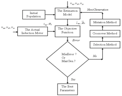
A. An initial population creation of parameters. It is

[image:3.595.73.271.135.290.2]

based on randomness.

P

₀₀ is generated with randomly selected individuals. Each individual parameter is constrained by the following condition

Fig. 1 The algorithm of the estimation model programming

max

min

P

≤

_ij

≥

,

i

=

1 ,

2 ,...,

n

and

j

=

1 ,

2 ,...,

m

where

P

_minand

P

_max are the limits of the parameter vector values.

n

is maximum numbers of generation and

m

_{is number of parameters or variables. After randomly} generating initial population, they will be transformed into binary number. Simultaneously, the ABC-reference frame voltages (

v

_sa

,

v

_sb

,

v

_sc) are sent to the estimation model. The estimation model produces dq0-reference frame currents (

i

sd

,

i

sq

,

i

s₀) and rotor speeds (

ω

r). The

currents are transformed back into ABC-reference frame

currents and the rotor speeds are transformed into radian per second unit. The only 1 stator phase current and rotor speed are used to estimate the parameters by which they are used to calculate the error (Eq. 16) by comparing them with the measured currents and the rotor speeds collected from the induction motor

B. Evaluation Operation. Firstly, the binary number of

each parameter will be transformed back into decimal number. Then, each individual is used to calculate the error from objective function. The error of objective function can be shown as

) , ( ) , ( ) ,

(ngen t Y ngen t Y ngen t

E = − (15)

where

Y

(

t

)

=

[

i

_sa

ω

_r

]

and

Y

(

t

)

=

[

i

sa

ω

r

]

where vectors

Y

are measured data and

Y

are estimated data.

∑

=

Λ = max

0

) , ( ) , ( )

( T

t

T

t ngen E t ngen E ngen

Fitness (16)

where

Λ

is a unit matrix,

t

is sampling time

C. GA procedures: selection, Crossover, Mutation Operation. The Probability of Crossover,

P

_c is 0.80 and

Probability of Mutation,

P

_m is 0.001in this paper. The next generation (offspring) from their parent will be produced from this GA operation. They are used to calculate for next iteration. The program will be terminated if the minimal error from objective function or the maximal number of generation is reached.

IV. SIMULATION STUDY

[image:3.595.309.546.343.782.2]

A program of the motor parameters estimation is developed in Matlab code. It is important to define the range of parameters -

P

_minand

P

_max to start the computation. In the simulation study, the maximum generation number was set up at 200 and the population size equal to 10. The measured data of stator voltages, currents and rotor speeds were collected from steady state period. Simulation test were conducted with 3 different types of the induction motors. The specifications of each motor are listed in TABLE I. The test of each motor was conducted with 5 different load levels (0%, 25%, 50%, 75% and 100% of full load). The results of the estimated parameters for the simulations are shown in Table II.-IV.

TABLE I.

The specifications of simulated induction motors

TABLE II.

The results of parameter estimation on different load from Motor 1

Motor 1

s

R

x

_ls

R

_r

x

_lr

x

_m

Real V. 2.2530 0.1000 2.3510 0.9000 40.8000 0 % Load 2.2900 0.1040 2.3900 0.8980 40.0230 Error (%) 1.6423 4.0000 1.6589 0.2222 1.9044 25 % Load 2.2500 0.0970 2.3500 0.8850 40.3010 Error (%) 0.1332 3.0000 0.0425 1.6667 1.2230 50% Load 2.2300 0.1050 2.3500 0.9370 40.2980 Error (%) 1.0209 5.0000 0.0425 4.1111 1.2304 75% Load 2.2100 0.0980 2.3503 0.9140 40.7190 Error (%) 1.9086 2.0000 0.0298 1.5556 0.1985

100%Load 2.2290 0.1050 2.3000 0.9080 40.8000

Error (%) 1.0652 .0000 2.1693 0.8889 0

Unit: Ohm (Ω)

TABLE III.

Motor 2

s

R

x

_ls

R

_r

x

_lr

x

_m

Real V. 0.0453 0.0775 0.0222 0.0322 2.0420 0% Load 0.0408 0.0788 0.0200 0.0360 2.0288 Error(%) 9.9338 1.6774 9.9099 11.8012 0.6464 25%Load 0.0408 0.0778 0.0200 0.0339 2.0458 Error(%) 9.9338 0.3871 9.9099 5.2795 0.1861 50%Load 0.0448 0.0801 0.0200 0.0310 2.0208 Error(%) 1.1038 3.3548 9.9099 3.7267 1.0382 75% Load 0.0408 0.0798 0.0200 0.0320 2.0418 Error (%) 9.9338 2.9677 9.9099 0.6211 0.0098 100%Load 0.0408 0.0717 0.0200 0.0310 2.0488 Error (%) 9.9338 7.4839 9.9099 3.7267 0.3330

Unit: Ohm (Ω)

(4)

TABLE IV.

Motor 3

s

R

x

ls

R

r

x

lr

x

m Real V. 3.3500 2.1803 1.9900 2.1803 51.4373 0% Load 3.3450 2.1292 1.9210 2.1232 51.3186 Error(%) 0.1493 2.3437 3.4673 2.6189 0.2308 25%Load 3.3150 2.2662 1.9410 2.2172 51.2906 Error(%) 1.0448 3.9398 2.4623 1.6924 0.2852 50%Load 3.3550 2.1989 2.0310 2.1002 51.6086 Error(%) 0.1493 0.8531 2.0603 3.6738 0.3330 75% Load 3.3550 2.1452 1.9910 2.1302 51.3272 Error (%) 0.1493 1.6099 0.0503 2.2978 0.2140 100%Load 3.4350 2.3452 1.9410 2.2522 51.2206 Error (%) 2.5373 7.5632 2.4623 3.2977 0.4213

Unit: Ohm (Ω)

The results in simulation test show good accuracy of estimation. The population and generation sizes can help improve the accuracy, but it also increase the time of the estimation. However, this test has been done without voltage unbalance and measurement noises. These factors can affect the accuracy of estimation

V. EXPERIMENTAL VERIFICATION

Having validated the proposed method on the simulations, the method has now been tested on the experimental cases. The experimental setup is shown Fig. 2. The setup consists of an induction motor with load cell with a facility to collect the 3-phase current - voltage signals and rotor speed decoder data directly to the PC at the user define sampling frequency. The technical specifications of the induction motor used in this experiment are listed in TABLE V. Motor 1 (M1) and 2 (M2) in TABLE V. are identical motors, Motor 1 has the rotor fault only and Motor 2 is healthy but the stator fault can be simulated by the 5 turn short circuit, 10 turn short circuit and 15 turn short circuit. The load cell is nothing but a DC generator. The load in the induction motor can be adjusted by changing field resistance of the DC generator. Hence the experiments were conducted at different load levels. The data were collected at the sampling frequency of 1280 samples/s. Initially the values of the parameters have been estimated by the method suggested by Mutlue et. al. [7] using the specifications shown in the nameplate of the motor. Thus, these data are listed below and assumed these parameters reflecting as the healthy status of the motor.

s

R

= 1.7056 Ω,

R

_r= 1.0020 Ω,

x

_ls= 0.8553 Ω,

x

_lr= 0.8553 Ω,

x

_m= 40.1854 Ω

TABLE V.

The specifications of experimental induction motors

M1= Rotor Fault Motor, M2 = Healthy and Stator Fault Motor

Fig. 2 Schematic of the experimental setup

This test, maximum generation was set up at 200 and population number as 10. The data are also collected from 5 different load levels and 3 different conditions (healthy, rotor fault and stator faults). The stator fault motor (Motor 2) can be divided into open circuit (healthy), 5 turn short circuit, 10 turn short circuit, 15 turn short circuit. During experiments, several sets of the stator voltage, current and rotor speed data were collected at different times. The average values of the estimation results will be expressed. The estimated results are shown in TABLE VI.-X. It can be seen from all tables, the estimated parameters for the healthy case are close to the actual values irrespective of load conditions. For the faulty stators, the estimated parameters related to the stator only are decreasing and the rotor parameters are remain close to the healthy values, and similar observations have been made for the rotor faults. Hence the suggested approach is robust for the experimental cases as well where the signals are expected to have some measurement noise. Unfortunately, both the rotor and stator faults were not simulated simultaneously in the experiments to further enhance the confidence level in the suggested approach.

TABLE VI.

The estimated parameters for the experimental case (0 % Load)

25%

Load

R

s

x

ls

R

r

x

lr

x

m

Actual Value

1.7056 0.8553 1.0020 0.8553 40.1854

Estimated Parameters

Healthy 1.5744 0.9577 0.9170 0.8344 40.2353 5 Turn

Short 0.8654 0.6944 0.9554 0.8656 40.0665

10 Turn Short

0.5776 0.4875 0.8944 0.8767 40.1646

15 Turn Short

0.3355 0.3233 1.0436 0.8891 40.3640

Broken

Bars 1.5500 0.9945 1.5237 1.2741 40.2233

Unit: Ohm (Ω)

Phase Power Voltages f PF

(5)

TABLE VII.

25%

Load

R

s

x

ls

R

r

x

lr

x

m

Actual

Value 1.7056 0.8553 1.0020 0.8553 40.1854

Healthy 1.5779 0.9232 0.9510 0.8461 40.1403 5 Turn

Short

0.7790 0.7454 0.9944 0.8901 40.2800

10 Turn Short

0.5906 0.4544 0.9875 0.8362 40.1098

15 Turn Short

0.3013 0.3112 0.9233 0.8990 40.0435

Broken Bars

1.5566 0.9237 1.5345 1.3211 40.2443

Unit: Ohm (Ω)

TABLE VIII.

50%

Load

R

s

x

ls

R

r

x

lr

x

m

Actual

Value 1.7056 0.8553 1.0020 0.8553 40.1854

Healthy 1.5912 0.9170 0.9577 0.8476 40.2353 5 Turn

Short

0.8654 0.6450 0.9446 0.8487 40.0654

10 Turn Short

0.5776 0.4988 0.9385 0.8590 40.0558

15 Turn Short

0.3155 0.2806 0.9243 0.8566 40.2774

Broken Bars

1.5632 0.9237 1.4931 1.3351 40.1567

Unit: Ohm (Ω)

TABLE IX.

75%

Load

R

s

x

ls

R

r

x

lr

x

m

Actual Value

1.7056 0.8553 1.0020 0.8553 40.1854

Healthy 1.5904 0.9457 0.9489 0.8344 40.2333 5 Turn

Short

0.8790 0.6309 0.9409 0.8211 40.1980

10 Turn

Short 0.5089 0.4342 0.9487 0.8598 40.1043

15 Turn Short

0.3240 0.3036 0.9300 0.8133 40.1040

Broken Bars

1.5560 0.9001 1.3945 1.2922 40.0031

Unit: Ohm (Ω)

TABLE X.

100%

Load

R

s

x

ls

R

r

x

lr

x

m

Actual

Value 1.7056 0.8553 1.0020 0.8553 40.1854

Healthy 1.5766 0.9170 0.9577 0.8795 40.0879 5 Turn

Short

0.9104 0.6554 0.9934 0.8370 40.2341

10 Turn Short

0.5640 0.4944 0.9671 0.8297 40.1754

15 Turn Short

0.3046 0.2896 0.9473 0.8534 40.0233

Broken Bars

[image:5.595.312.541.297.512.2]

1.5500 0.9257 1.3730 1.2678 40.0223

Fig. 3-4 show typical comparison of the stator phase current and rotor speeds both the measured and the estimated data during iterative process. The steady state period of the data are used while estimation.

Fig. 3 A typical comparisons of the measured and the estimated stator phase current from phase A

[image:5.595.316.526.653.735.2]

Fig. 4 The rotor speed from measured and estimated data

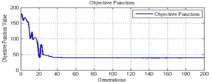
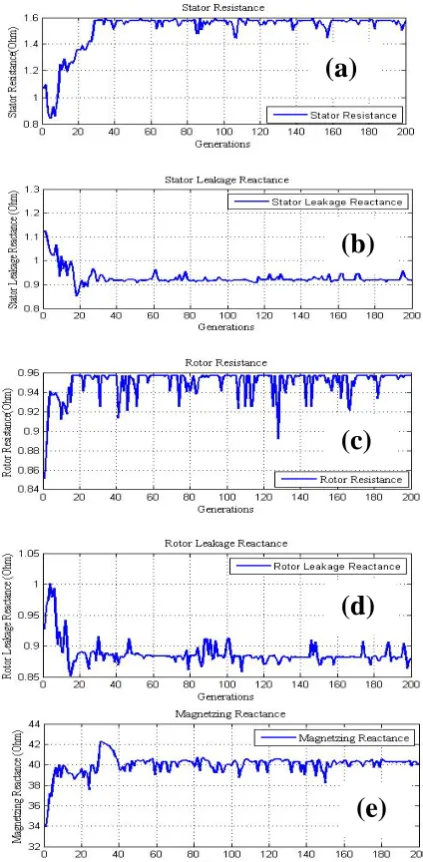
Fig. 5 shows the plotting of the Objective Function with Generation for the healthy Motor-2 at 100% load during GA convergence. Fig. 6 shows the typical plots of the parameter estimation at each generation for the healthy Induction Motor 2 at 100% load for the experimental case. There is small fluctuation in the estimated parameters has been observed with generations. However, fluctuation is always around the mean position for all the 5 parameters. This also indicates there is no divergence in the estimation for the experimental case as well.

(6)

[image:6.595.66.278.70.502.2]

Fig. 10 Parameters estimation vs Generation for the healthy Experimental Motor-2 at 100% load;

(a)

R

_s, (b)

x

_ls (c)

R

_r (d)

x

_lr and (e)

x

_m

VI. CONCLUSIONS

A model is arranged from the flux linkage models and torque model of a squirrel-cage induction motor. The proposed GA method is applies as a key technique to estimates the motor parameters: stator and rotor resistance, stator and rotor reactance, and magnetizing reactance. The only 2 measurements (stator phase current and rotor speed) during the machine normal operation were used as the input data. The simulations were used to evaluate the proposed method and then the method has further been validated through the experiments on the induction motors. The motor faults (stator and rotor faults) can be predicted by observing the change in the parameters. The voltage unbalances from the motor installed at site in some cases may slightly affect the accuracy of the estimation. Thus, the further development is also under way

REFERENCES

[1] Treetrong J., Zhang K., Fan Y. E., Gu F. and Ball A., Monitoring electric motors based on parameters identification techniques, Second World Congress on Engineering Asset Management and Fourth International Conference on condition monitoring, Harrogate, 2007, UK

[2] Horga V., Onea A., and Ratoi M., Parameter Estimation of Induction Motor Based on Continuous Time Model’, Proceedings of the 6th WSEAS International Conference on Simulation, Modelling and Optimization, Lisbon, Portugal, September 2006, 513-518

[3] Koubaa Y., Recursive identification of induction motor parameters, Simulation Modeling Practice and Theory, 2004, v. 12, 363–381

[4] Velazquez S. C., Palomares R. A., and Segura A. N., Speed Estimation for an Induction Motor Using the Extended Kalman Filter, Proceedings of the 14th International Conference on Electronics, Communications and Computers (CONIELECOMP’04), 2004

[5] Barut M., Bogosyan S., and Gokasan M., Speed-Sensorless Estimation for Induction Motors Using Extended Kalman Filters, Industrial Electronics, IEEE Transaction on, v. 54-1, 2007, 272-280

[6] Nangsue P., Pillay P., and Conry S. E., Evolutionary Algorithm for Industrial Motor Parameter Determination, Energy Conversion, IEEE Transaction on, v 14-3, 1999, 447-453

[7] Mutluer M. Bilgin O. and Cunkas M., Parameter Determination of Induction Machines by Hybrid Genetic Algorithms, KES 2007/WIRN 2007, Part I, 2007, 116 – 124

[8] Huang K. S., Kent W., Wu Q. H. and Turner D.R., Parameter Identification of an induction Machine Using Genetic Algorithms, Proceeding of the 1999 IEEE International Symposium on Computer Aid Control System Design, Hawai, 1999, USA [9] Huang K. S., Kent W., Wu Q. H. and Turner D.R., Effective

Identification of Induction Motor Parameters Based on Fewer Measurements, Energy Conversion, IEEE Transaction on, v. 17-1, 2002, 55-60

[10] Ong C. M., Dynamic Simulation of Electric Machinery using Matlab/Simulink (Prentice Hall Book, 1998)

[11] Krause P. C., Analysis of Electric Machinery, (McGraw-Hill Book Company, 1986)

[12] Goldberg D. E (1989), Genetic Algorithm in Search, Optimization, and Machine Learning (Addison-Wesley, 1989) [13] Eiben A. E. and Smith J. E., Introduction to Evolutionary