Efficient and Expressive Knowledge Base Completion Using Subgraph Feature Extraction

Efficient and Expressive Knowledge Base Completion

Using Subgraph Feature Extraction

Matt Gardner and Tom Mitchell Carnegie Mellon University

[email protected], [email protected]

Abstract

We explore some of the practicalities of using random walk inference meth-ods, such as the Path Ranking Algorithm (PRA), for the task of knowledge base completion. We show that the random walk probabilities computed (at great ex-pense) by PRA provide no discernible benefit to performance on this task, so they can safely be dropped. This allows us to define a simpler algorithm for gener-ating feature matrices from graphs, which we call subgraph feature extraction (SFE). In addition to being conceptually simpler than PRA, SFE is much more efficient, re-ducing computation by an order of mag-nitude, and more expressive, allowing for much richer features than paths between two nodes in a graph. We show experi-mentally that this technique gives substan-tially better performance than PRA and its variants, improving mean average preci-sion from .432 to .528 on a knowledge base completion task using the NELL KB.

1 Introduction

Knowledge bases (KBs), such as Freebase (Bol-lacker et al., 2008), NELL (Mitchell et al., 2015), and DBPedia (Mendes et al., 2012) contain large collections of facts about things, people, and places in the world. These knowledge bases are useful for various tasks, including training rela-tion extractors and semantic parsers (Hoffmann et al., 2011; Krishnamurthy and Mitchell, 2012), and question answering (Berant et al., 2013). While these knowledge bases may be very large, they are still quite incomplete, missing large percentages of facts about common or popular entities (West et al., 2014; Choi et al., 2015). The task of knowl-edge base completion—filling in missing facts by

examining the facts already in the KB, or by look-ing in a corpus—is one attempt to mitigate the problems of this knowledge sparsity.

In this work we examine one method for performing knowledge base completion that is currently in use: the Path Ranking Algorithm (PRA) (Lao et al., 2011; Dong et al., 2014). PRA is a method for performing link prediction in a graph with labeled edges by computing feature matrices over node pairs in the graph. The method has a strong connection to logical inference (Gard-ner et al., 2015), as the feature space considered by PRA consists of a restricted class of horn clauses found in the graph. While PRA can be applied to any link prediction task in a graph, its primary use has been in KB completion (Lao et al., 2012; Gardner et al., 2013; Gardner et al., 2014).

PRA is a two-step process, where the first step finds potential path types between node pairs to use as features in a statistical model, and the sec-ond step computes random walk probabilities as-sociated with each path type and node pair (these are the values in a feature matrix). This second step is very computationally intensive, requiring time proportional to the average out-degree of the graph to the power of the path length foreach cell in the computed feature matrix. In this paper we consider whether this computational effort is well-spent, or whether we might more profitably spend computation in other ways. We propose a new way of generating feature matrices over node pairs in a graph that aims to improve both the efficiency and the expressivity of the model relative to PRA.

Our technique, which we call subgraph fea-ture extraction(SFE), is similar to only doing the first step of PRA. Given a set of node pairs in a graph, we first do a local search to characterize the graph around each node. We then run a set of feature extractors over these local subgraphs to obtain feature vectors for each node pair. In the simplest case, where the feature extractors only

look for paths connecting the two nodes, the fea-ture space is equivalent to PRA’s, and this is the same as running PRA and binarizing the resultant feature vectors. However, because we do not have to compute random walk probabilities associated with each path type in the feature matrix, we can extract much more expressive features, including features which are not representable as paths in the graph at all. In addition, we can do a more exhaus-tive search to characterize the local graph, using a breadth-first search instead of random walks. SFE is a much simpler method than PRA for obtaining feature matrices over node pairs in a graph. De-spite its simplicity, however, we show experimen-tally that it substantially outperforms PRA, both in terms of running time and prediction performance. SFE decreases running time over PRA by an order of magnitude, it improves mean average precision from .432 to .528 on the NELL KB, and it im-proves mean reciprocal rank from .850 to .933.

In the remainder of this paper, we first describe PRA in more detail. We then situate our meth-ods in the context of related work, and provide ad-ditional experimental motivation for the improve-ments described in this paper. We then formally define SFE and the feature extractors we used, and finally we present an experimental compari-son between PRA and SFE on the NELL KB. The code and data used in this paper is available at http://rtw.ml.cmu.edu/emnlp2015 sfe/.

2 The Path Ranking Algorithm

The path ranking algorithm was introduced by Lao and Cohen (2010). It is a two-step process for gen-erating a feature matrix over node pairs in a graph. The first step finds a set of potentially useful path types that connect the node pairs, which become the columns of the feature matrix. The second step then computes the values in the feature matrix by finding random walk probabilities as described be-low. Once the feature matrix has been computed, it can be used with whatever classification model is desired (or even incorporated as one of many factors in a structured prediction model), though almost all prior work with PRA simply uses logis-tic regression.

More formally, consider a graph G with nodes

N, edgesE, and edge labelsR, and a set of node pairs (sj,tj)∈ Dthat are instances of some rela-tionship of interest. PRA will generate a feature vector for each (sj,tj) pair, where each feature is

some sequence of edge labels -e1-e2-. . .-el-. If the edge sequence, orpath type, corresponding to the feature exists between the source and target nodes in the graph, the value of that feature in the feature vector will be non-zero.

Because the feature space considered by PRA is so large,1 _{and because computing the feature}

values is so computationally intensive, the first step PRA must perform isfeature selection, which is done using random walks over the graph. In this step of PRA, we find path types π that are likely to be useful in predicting new instances of the relation represented by the input node pairs. These path types are found by performing random walks on the graph G starting at the source and target nodes inDand recording which paths con-nect some source node with its target.2 _{Note that}

these aretwo-sided,unconstrainedrandom walks: the walks from sources and targets can be joined on intermediate nodes to get a larger set of paths that connect the source and target nodes. Once connectivity statistics have been computed in this way,kpath types are selected as features. Lao et al. (2011) use measures of the precision and recall of each feature in this selection, while Gardner et al. (2014) simply pick those most frequently seen. Once a set of path features has been selected, the second step of PRA is to compute values for each cell in the feature matrix. Recall that rows in this matrix correspond to node pairs, and the columns correspond to the path types found in the first step. The cell value assigned by PRA is the probability of arriving at the target node of a node pair, given that a random walk began at the source node and was constrained to follow the path type: p(t|s, π). There are several ways of computing this probability. The most straightforward method is to use a path-constrained breadth-first search to exhaustively enumerate all possible targets given a source node and a path type, count how frequently each target is seen, and normalize the distribution. This calculates the desired probability exactly, but at the cost of doing a breadth-first search (with

1_{The feature space consists of the set of all possible edge} label sequences, with cardinality Pl_i=1|R|i_{, assuming a} boundlon the maximum path length.

complexity proportional to the average per-edge-label out-degree to the power of the path length) per source node per path type.

There are three methods that can potentially re-duce the computational complexity of this proba-bility calculation. The first is to use random walks to approximate the probability via rejection sam-pling: for each path type and source node, a num-ber of random walks are performed, attempting to follow the edge sequence corresponding to the path type. If a node is reached where it is no longer possible to follow the path type, the ran-dom walk is restarted. This does not reduce the time necessary to get an arbitrarily good approxi-mation, but it does allow us to decrease computa-tion time, even getting a fixed complexity, at the cost of accepting some error in our probability es-timates. Second, Lao (2012) showed that when the target node of a query is known, the exponent can be cut in half by using a two-sided BFS. In this method, some careful bookkeeping is done with dynamic programming such that the probability can be computed correctly when the two-sided search meets at an intermediate node. Lao’s dy-namic programming technique is only applicable when the target node is known, however, and only cuts the exponent in half—this is still quite compu-tationally intensive. Lastly, we could replace the BFS with a multiplication of adjacency matrices, which performs the same computation. The effi-ciency gain comes from the fact that we can just do the multiplication once per path type, instead of once per path type per source node. However, to correctly compute the probabilities for a (source, target) pair, we need to exclude from the graph the edge connecting that training instance. This means that the matrix computed for each path typeshould be different for each training instance, and so we either lose our efficiency gain or we accept incor-rect probability estimates. In this work we use the rejection sampling technique.

As mentioned above, once the feature matrix has been computed in the second step of PRA, one can use any kind of classifier desired to learn a model and make predictions on test data.

3 Related Work

The task of knowledge base completion has seen a lot of attention in recent years, with entire work-shops devoted to it (Suchanek et al., 2013). We will touch on three broad categories related to KB

completion: the task of relation extraction, embed-ding methods for KB completion, and graph meth-ods for KB completion.

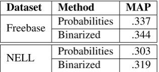
Dataset Method MAP Freebase Probabilities_Binarized .337_.344

NELL Probabilities_Binarized .303_.319

Table 1: Using binary feature values instead of random walk probabilities gives statistically in-distinguishable performance. Thep-value on the Freebase data is .55, while it is .25 for NELL.

Graph-based methods for KB completion. A separate line of research into KB completion can be broadly construed as performing some kind of inference over graphs in order to predict missing instances in a knowledge base. Markov logic net-works (Richardson and Domingos, 2006) fall into this category, as does ProPPR (Wang et al., 2013) and many other logic-based systems. PRA, the main subject of this paper, also fits in this line of work. Work specifically with PRA has ranged from incorporating a parsed corpus as additional evidence when doing random walk inference (Lao et al., 2012), to introducing better representations of the text corpus (Gardner et al., 2013; Gardner et al., 2014), and using PRA in a broader context as part of Google’s Knowledge Vault (Dong et al., 2014). An interesting piece of work that combines embedding methods with graph-based methods is that of Neelakantan et al. (2015), which uses a re-cursive neural network to create embedded repre-sentations of PRA-style paths.

4 Motivation

We motivate our modifications to PRA with three observations. First, it appears that binarizing the feature matrix produced by PRA, removing most of the information gained in PRA’s second step, has no significant impact on prediction perfor-mance in knowledge base completion tasks. We show this on the NELL KB and the Freebase KB in Table 1.3 _{The fact that random walk probabilities}

carry no additional information for this task over binary features is surprising, and it shows that the second step of PRA spends a lot of its computation for no discernible gain in performance.

Second, Neelakantan et al. (2015) presented

ex-3_{The NELL data and experimental protocol is described} in Section 6.1. The Freebase data consists of 24 relations from the Freebase KB; we used the same data used by Gard-ner et al. (2014).

periments showing a substantial increase in perfor-mance from using a much larger set of features in a PRA-like model.4 _{All of their experiments used}

binary features, so this is not a direct comparison of random walk probabilities versus binarized fea-tures, but it shows that increasing the feature size beyond the point that is computationally feasible with random walk probabilities seems useful. Ad-ditionally, they showed that using path bigram fea-tures, where each sequential pair of edges types in each path was added as an additional feature to the model, gave a significant increase in performance. These kind of features are not representable in the traditional formulation of PRA.

Lastly, the method used to compute the random walk probabilities—rejection sampling—makes the inclusion of more expressive features problem-atic. Consider the path bigrams mentioned above; one could conceivably compute a probability for a path type that only specifies that the last edge type in the path must ber, but it would be incredibly inefficient with rejection sampling, as most of the samples would end up rejected (leaving aside the additional issues of an unspecified path length). In contrast, if the features simply signify whether a particular path type exists in the graph, without any associated probability, these kinds of features are very easy to compute.

Given this motivation, our work attempts to im-prove both the efficiency and the expressivity of PRA by removing the second step of the algo-rithm. Efficiency is improved because the sec-ond step is the most computationally expensive, and expressivity is improved by allowing features that cannot be reasonably computed with rejec-tion sampling. We show experimentally that the techniques we introduce do indeed improve per-formance quite substantially.

5 Subgraph Feature Extraction

In this section we discuss how SFE constructs fea-ture matrices over node pairs in a graph using just a single search over the graph for each node (which is comparable to only using the first step of PRA). As outlined in Section 2, the first step of PRA does a series of random walks from each source and target node (sj, tj) in a datasetD. In

PRA these random walks are used to find a rela-tively small set of potentially useful path types for which more specific random walk probabilities are then computed, at great expense. In our method, subgraph feature extraction (SFE), we stop after this first set of random walks and instead construct a binary feature matrix.

More formally, for each node n in the data (wherencould be either a source node or a target node), SFE constructs a subgraph centered around that node using k random walks. Each random walk that leavesn follows some path typeπ and ends at some intermediate node i. We keep all of these (π,i) pairs as the characterization of the subgraph aroundn, and we will refer to this sub-graph as Gn. To construct a feature vector for a source-target pair (sj, tj), SFE takes the sub-graphs Gsj andGtj and merges them on the in-termediate nodes i. That is, if an intermediate nodeiis present in bothGsj andGtj, SFE takes the path typesπ corresponding toiand combines them (reversing the path type coming from the tar-get node tj). If some intermediate node for the sourcesjhappens to betj, no combination of path types is necessary (and similarly if an intermediate node for the targettjissj—the path only needs to be reversed in this case). This creates a feature space that is exactly the same as that constructed by PRA: sequences of edge types that connect a source node to a target node. To construct the fea-ture vector SFE just takes all of these combined path types as binary features for (sj, tj). Note, however, that we need not restrict ourselves to only using the same feature space as PRA; Sec-tion 5.1 will examine extracting more expressive features from these subgraphs.

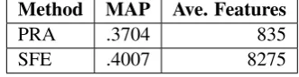
This method for generating a feature matrix over node pairs in a graph is much simpler and less computationally expensive than PRA, and from looking at Table 1 we would expect that it would perform on par with PRA with drastically reduced computation costs. Some experimentation shows that it is not that simple. Table 2 shows a com-parison between PRA and SFE on 10 NELL rela-tions.5 _{SFE has a higher mean average precision,}

but the difference is not statistically significant. There is a large variance in SFE’s performance, and on some relations PRA performs better.

We examined the feature matrices computed

5_{The data and evaluation methods are described more} fully in Section 6.1. These experiments were conducted on a different development split of the same data.

Method MAP Ave. Features

PRA .3704 835

SFE .4007 8275

Table 2: Comparison of PRA and SFE on 10 NELL relations. The difference shown is not sta-tistically significant.

by these methods and discovered that the reason for the inconsistency of SFE’s improvement is because its random walks are all unconstrained. Consider the case of a node with a very high de-gree, say 1000. If we only do 200 random walks from this node, we cannot possibly get a complete characterization of the graph even one step away from the node. If a particularly informative path is

<CITYINSTATE, STATEINCOUNTRY>, and both the city from which a random walk starts and the intermediate state node have very high degree, the probability of actually finding this path type using unconstrained random walks is quite low. This is the benefit gained by thepath-constrainedrandom walks performed by PRA; PRA leverages training instances with relatively low degree and aggrega-tion across a large number of instances to find path types that are potentially useful. Once they are found, significant computational effort goes into discovering whether each path type exists forall (s, t) pairs. It is this computational effort that allows the path type<CITYINSTATE, STATEIN -COUNTRY> to have a non-zero value even for very highly connected nodes.

Method MAP Ave. Features Time

PRA .3704 835 44 min.

SFE-RW .4007 8275 6 min.

SFE-BFS .4799 237853 5 min.

Table 3: Comparison of PRA and SFE (with PRA-style features) on 10 NELL relations. SFE-RW is not statistically better than PRA, but SFE-BFS is (p <0.05).

node; we just do not continue searching if the out-degree of a particular edge type is too high.

When using a BFS instead of random walks to obtain the subgraphs Gsj andGtj for each node pair, we saw a dramatic increase in the number of path type features found and a substantial increase in performance.6 _{These results are shown in}

Ta-ble 3; SFE-RW is our SFE implementation using random walks, and SFE-BFS uses a BFS.

5.1 More expressive features

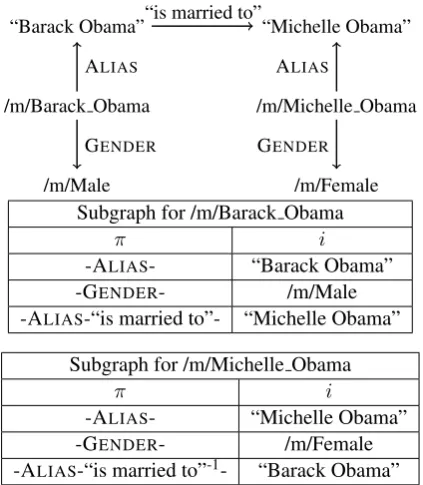
The description above shows how to recreate the feature space used by PRA using our simpler sub-graph feature extraction technique. As we have mentioned, however, we need not restrict our-selves to merely recreating PRA’s feature space. Eliminating random walk probabilities allows us to extract a much richer set of features from the subgraphs around each node, and here we present the feature extractors we have experimented with. Figure 1 contains an example graph that we will refer to when describing these features.

PRA-style features. We explained these fea-tures in Section 5, but we repeat them here for con-sistency, and use the example to make the feature extraction process more clear. Relying on the no-tation introduced earlier, these features are gener-ated by intersecting the subgraphsGs andGt on the intermediate nodes. That is, when the sub-graphs share an intermediate node, we combine the path types found from the source and target to that node. In the example in Figure 1, there are two common intermediate nodes (“Barack Obama” and “Michelle Obama”), and combining the path types corresponding to those nodes gives the same path type: -ALIAS-“is married to”-ALIAS-1-.

Path bigram features. In Section 4, we mentioned that Neelakantan et al. (2015) experi-mented with using path bigrams as features. We

6_{One should not read too much into the decrease in} run-ning time between SFE-RW and SFE-BFS, however, as it was mostly an implementation detail.

/m/Barack Obama /m/Michelle Obama “Barack Obama” “Michelle Obama”

/m/Male /m/Female ALIAS

GENDER

ALIAS

GENDER “is married to”

Subgraph for /m/Barack Obama

π i

-ALIAS- “Barack Obama”

-GENDER- /m/Male

-ALIAS-“is married to”- “Michelle Obama”

Subgraph for /m/Michelle Obama

π i

-ALIAS- “Michelle Obama”

-GENDER- /m/Female

-ALIAS-“is married to”-1- “Barack Obama”

Figure 1: An example graph, with subgraphs ex-tracted for two nodes.

include those features here as well. For any path

πbetween a source nodesand a target nodet, we create a feature for each relation bigram in the path type. In the example in Figure 1, this would result in the features “BIGRAM:@START@-ALIAS”, “BIGRAM:ALIAS-is married to”, “BIGRAM:is married to-ALIAS”, and “BIGRAM:ALIAS -@END@”.

One-sided features. We useone-sided pathto describe a sequence of edges that starts at a source or target node in the data, but does not necessarily terminate at a corresponding target or source node, as PRA features do. Following the notation intro-duced in Section 5, we use as features each (π,

i) pair in the subgraph characterizations Gs and

Gt, along with whether the feature came from the source node or the target node. The motivation for these one-sided path types is to better model which sources and targets are good candidates for participating in a particular relation. For example, not all cities participate in the relation CITYCAPI -TALOFCOUNTRY, even though the domain of the relation is all cities. A city that has a large number of sports teams may be more likely to be a capi-tal city, and these one-sided features could easily capture that kind of information.

“SOURCE:-ALIAS-:Barack Obama”, and “SOURCE:-ALIAS-is married to-:Michelle Obama”.

One-sided feature comparisons. We can ex-pand on the one-sided features introduced above by allowing for comparisons of these features in certain circumstances. For example, if both the source and target nodes have an age or gender en-coded in the graph, we might profitably use com-parisons of these values to make better predictions. Drawing again on the notation from Section 5, we can formalize these features as analogous to the pairwise PRA features. To get the PRA features, we intersect the intermediate nodes i

from the subgraphsGs andGt, and combine the path typesπ when we find common intermediate nodes. To get these comparison features, we in-stead intersect the subgraphs on the path types, and combine the intermediate nodes when there are common path types. That is, if we see a com-mon path type, such as -GENDER-, we will con-struct a feature representing a comparison between the intermediate node for the source and the target. If the values are the same, this information can be captured with a PRA feature, but it cannot be eas-ily captured by PRA when the values are different. In the example in Figure 1, there are two common path types: -ALIAS-, and -GENDER . The feature generated from the path type -GENDER- would be “COMPARISON:-GENDER -:/m/Male:/m/Female”.

Vector space similarity features. Gardner et al. (2014) introduced a modification of PRA’s ran-dom walks to incorporate vector space similarity between the relations in the graph. On the data they were using, a graph that combined a formal knowledge base with textual relations extracted from text, they found that this technique gave a substantial performance improvement. The vector space random walks only affected the second step of PRA, however, and we have removed that step in SFE. While it is not as conceptually clean as the vector space random walks, we can obtain a similar effect with a simple feature transformation using the vectors for each relation. We obtain vec-tor representations of relations through facvec-toriza- factoriza-tion of the knowledge base tensor as did Gardner et al., and replace each edge type in a PRA-style path with edges that are similar to it in the vec-tor space. We also introduce a special “any edge” symbol, and say that all other edge types are

simi-lar to this edge type.

To reduce the combinatorial explosion of the feature space that this feature extractor cre-ates, we only allow replacing one relation at a time with a similar relation. In the ex-ample graph in Figure 1, and assuming that “spouse of” is found to be similar to “is mar-ried to”, some of the features extracted would be the following: “VECSIM:-ALIAS-is married to-ALIAS-”, “VECSIM:-ALIAS-spouse of-ALIAS-”, “VECSIM:-ALIAS-@ANY REL@-ALIAS-”, and “VECSIM:-@ANY REL@-is married to-ALIAS -”. Note that the first of those features, “VECSIM:-ALIAS-is married to-ALIAS-”, is necessary even though it just duplicates the original PRA-style feature. This allows path types with different but similar relations to generate the same features.

Any-Relation features. It turns out that much of the benefit gained from Gardner et al.’s vector space similarity features came from allowing any path type that used a surface edge to match any other surface edge with non-zero probability.7 _{To test whether the vector space}

similarity features give us any benefit over just replacing relations with dummy symbols, we add a feature extractor that is identical to the one above, assuming an empty vector similarity mapping. The features extracted from Figure 1 would thus be “ANYREL:-@ANY REL@-is married to-ALIAS”, “ANYREL:-ALIAS -@ANY REL@-ALIAS”, “ANYREL:-ALIAS-is married to-@ANY REL@”.

6 Experiments

Here we present experimental results evaluating the feature extractors we presented, and a com-parison between SFE and PRA. As we showed in Section 5 that using a breadth-first search to ob-tain subgraphs is superior to using random walks, all of the experiments presented here use the BFS implementation of SFE.

6.1 Data

To evaluate SFE and the feature extractors we in-troduced, we learned models for 10 relations in the NELL KB. We used the same data as Gardner et al. (2014), using both the formal KB relations and the surface relations extracted from text in our

graph. We used logistic regression with elastic net (L1 and L2) regularization. We tuned the L1 and L2 parameters for each method on a random de-velopment split of the data, then used a new split of the data to run the final tests presented here.

The evaluation metrics we use are mean aver-age precision (MAP) and mean reciprocal rank (MRR). We judge statistical significance using a paired permutation test, where the average preci-sion8_{on each relation is used as paired data.}

6.2 On Obtaining Negative Evidence

One important practical issue for most uses of PRA is the selection of negative examples for training a model. Typically a knowledge base only contains positive examples of a relation, and it is not clear a priori what the best method is for ob-taining negative evidence. Prior work with PRA makes a closed world assumption, treating any (s,

t) pair not seen in the knowledge base as a negative example. Negative instances are selected when performing the second step of PRA—if a random walk from a source ends at a target that is not a known correct target for that source, that source-target pair is used as a negative example.

SFE only scores (source, target) pairs; it has no mechanism similar to PRA’s that will find poten-tial targets given a source node. We thus need a new way of finding negative examples, both at training time and at test time. We used a simple technique to find negative examples from a graph given a set of positive examples, and we used this to obtain the training and testing data used in the experiments below. Our technique takes each source and target node in the given positive exam-ples and finds other nodes in the same category that are close in terms of personalized page rank (PPR). We then sample new (source, target) pairs from these lists of similar nodes, weighted by their PPR score (while also allowing the original source and target to be sampled). These become our neg-ative examples, both at training and at testing time. Because this is changing the negative evidence available to PRA at training time, we wanted to be sure we were not unfairly hindering PRA in our comparisons. If it is in fact better to let PRA find its own negative examples at training time, instead of the ones sampled based on personalized page rank, then we should let PRA get its own

nega-8_{Average precision is equivalent to the area under a} preci-sion/recall curve.

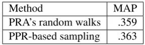
Method MAP

PRA’s random walks .359 PPR-based sampling .363

Table 4: Comparing methods for obtaining nega-tive evidence available at training time. The differ-ence seen is not statistically significant (p=.77).

tive evidence. We thus ran an experiment to see under which training regime PRA performs bet-ter. We created a test set with both positive and negative examples as described in the paragraph above, and at training time we compared two tech-niques: (1) letting PRA find its own negative ex-amples through its random walks, and (2) only using the negative examples selected by PPR. As can be seen in Table 4, the difference between the two training conditions is very small, and it is not statistically significant. Because there is no sig-nificant difference between the two conditions, in the experiments that follow we give both PRA and SFE the same training data, created through the PPR-based sampling technique described above. 6.3 Results

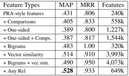
We first examine the effect of each of the fea-ture types introduced in Section 5.1. The results are shown in Table 5. We can see that, for this data, the comparisons and one-sided features did not improve performance (and the decreases are not statistically significant). Bigram features do appear to improve performance, though the im-provement was not consistent enough across rela-tions to achieve statistical significance. The vector similarity features do improve performance, with

p-values hovering right at 0.05 when comparing against only PRA features and PRA + bigram fea-tures. The any rel features, however, do statisti-cally improve over all other methods (p <= 0.01) except the PRA + vec sim result (p=.21).

Finally, we present a comparison between PRA, PRA with vector space random walks, and the best SFE result from the ablation study. This is shown in Table 6. SFE significantly outperforms PRA, both with and without the vector space random walks presented by Gardner et al. (2014).

6.4 Discussion

-Feature Types MAP MRR Features PRA-style features .431 .806 240k

+ Comparisons .405 .833 558k

+ One-sided .389 .800 1,227k

+ One-sided + Comps. .387 .817 1,544k

+ Bigrams .483 1.00 320k

+ Vector similarity .514 .910 3,993k + Bigrams + vec sim. .490 .950 4,073k

+ Any Rel .528 .933 649k

Table 5: SFE feature ablation study. All rows use PRA features. PRA + any rel is statistically better than all other methods except PRA + vec sim, and most of the other differences are not significant.

Method MAP MRR

PRA .362 .717

Vector space PRA .432 .850

SFE (PRA + any rel features) .528 .933

Table 6: Results of final comparison between SFE and PRA, with and without vector space similarity features. SFE is statistically better than both PRA methods (p <0.005).

WROTEBOOK, the textual relations used in this feature might be “wrote”, “describes in”, “writes in”, and “expresses in”. These are the same fea-ture types that PRA itself finds to have the high-est weight, also, though SFE finds many more of them than PRA does, as PRA has to do aggres-sive feature selection. For this particular dataset, where the graph consists of edges from a formal KB mixed with edges from extracted textual rela-tions, these kinds of features are by far the most useful, and most of the improvements seen by the additional feature types we used with SFE come from more compactly encoding these features.

For example, the path bigram features can en-code the fact that there exists a path from the source to the target that begins or ends with an ALIAS edge. This captures in just two features all path types of the form -ALIAS-[some textual relation]-ALIAS-1-, and those two bigram features are almost always the highest weighted features in models where they are used.

However, the bigram features do not capture those path types exactly. The Any-Rel features were designed in part specifically for this path type, and they capture it exactly with a single fea-ture. For all 10 relations, the feature “ANYREL:-ALIAS-@ANY REL@-ALIAS-1” is the highest

weighted feature. This is because, for the relations we experimented with, knowing that some rela-tionship is expressed in text between a particular pair of KB entities is a very strong indication of a single KB relation. There are only so many possi-ble relationships between cities and countries, for instance. These features are much less informative between entity types where more than one relation is possible, such as between people.

While the bigram and any-rel features capture succintly whether textual relations are present be-tween two entities, the one-sided features are more useful for determining whether an entity fits into the domain or range of a particular relation. We saw a few features that did this, capturing fine-grained entity types. Most of the features, how-ever, tended towards memorizing (and thus over-fitting) the training data, as these features con-tained the names of the training entities. We be-lieve this overfitting to be the main reason these features did not improve performance, along with the fact that the relations we tested do not need much domain or range modeling (as opposed to, e.g., SPOUSEOFor CITYCAPITALOFCOUNTRY).

7 Conclusion

We have explored several practical issues that arise when using the path ranking algorithm for knowledge base completion. An analysis of sev-eral of these issues led us to propose a sim-pler algorithm, which we called subgraph fea-ture extraction, which characterizes the subgraph around node pairs and extracts features from that subgraph. SFE is both significantly faster and performs better than PRA on this task. We showed experimentally that we can reduce run-ning time by an order of magnitude, while at the same time improving mean average preci-sion from .432 to .528 and mean reciprocal rank from .850 to .933. This thus constitutes the best published results for knowledge base com-pletion on NELL data. The code and data used in the experiments in this paper are available at http://rtw.ml.cmu.edu/emnlp2015 sfe/.

Acknowledgements

References

Jonathan Berant, Andrew Chou, Roy Frostig, and Percy Liang. 2013. Semantic parsing on freebase from question-answer pairs. In EMNLP, pages 1533– 1544.

Kurt Bollacker, Colin Evans, Praveen Paritosh, Tim Sturge, and Jamie Taylor. 2008. Freebase: a col-laboratively created graph database for structuring human knowledge. InProceedings of SIGMOD.

Antoine Bordes, Jason Weston, Ronan Collobert, Yoshua Bengio, et al. 2011. Learning structured embeddings of knowledge bases. InAAAI.

Antoine Bordes, Nicolas Usunier, Alberto Garcia-Duran, Jason Weston, and Oksana Yakhnenko. 2013. Translating embeddings for modeling multi-relational data. InAdvances in Neural Information Processing Systems, pages 2787–2795.

Kai-Wei Chang, Wen-tau Yih, Bishan Yang, and Christopher Meek. 2014. Typed tensor decom-position of knowledge bases for relation extrac-tion. In Proceedings of the 2014 Conference on Empirical Methods in Natural Language Processing (EMNLP), pages 1568–1579.

Eunsol Choi, Tom Kwiatkowski, and Luke Zettle-moyer. 2015. Scalable semantic parsing with partial ontologies. InProceedings of ACL.

Xin Dong, Evgeniy Gabrilovich, Geremy Heitz, Wilko Horn, Ni Lao, Kevin Murphy, Thomas Strohmann, Shaohua Sun, and Wei Zhang. 2014. Knowl-edge vault: A web-scale approach to probabilis-tic knowledge fusion. In Proceedings of the 20th ACM SIGKDD international conference on Knowl-edge discovery and data mining, pages 601–610. ACM.

Alberto Garc´ıa-Dur´an, Antoine Bordes, and Nicolas Usunier. 2014. Effective blending of two and three-way interactions for modeling multi-relational data.

In Machine Learning and Knowledge Discovery in

Databases, pages 434–449. Springer.

Matt Gardner, Partha Talukdar, Bryan Kisiel, and Tom Mitchell. 2013. Improving learning and infer-ence in a large knowledge-base using latent syntac-tic cues. InProceedings of EMNLP. Association for Computational Linguistics.

Matt Gardner, Partha Talukdar, Jayant Krishnamurthy, and Tom Mitchell. 2014. Incorporating vector space similarity in random walk inference over knowledge bases. InProceedings of EMNLP. Association for Computational Linguistics.

Matt Gardner, Partha Talukdar, and Tom Mitchell. 2015. Combining vector space embeddings with symbolic logical inference over open-domain text.

In2015 AAAI Spring Symposium Series.

Raphael Hoffmann, Congle Zhang, Xiao Ling, Luke Zettlemoyer, and Daniel S Weld. 2011. Knowledge-based weak supervision for information extraction of overlapping relations. InProceedings of the 49th Annual Meeting of the Association for Computa-tional Linguistics: Human Language Technologies-Volume 1, pages 541–550. Association for Compu-tational Linguistics.

Jayant Krishnamurthy and Tom M Mitchell. 2012. Weakly supervised training of semantic parsers. In Proceedings of the 2012 Joint Conference on Empir-ical Methods in Natural Language Processing and Computational Natural Language Learning, pages 754–765. Association for Computational Linguis-tics.

Ni Lao and William W Cohen. 2010. Relational re-trieval using a combination of path-constrained ran-dom walks.Machine learning, 81(1):53–67. Ni Lao, Tom Mitchell, and William W Cohen. 2011.

Random walk inference and learning in a large scale knowledge base. InProceedings of EMNLP. Asso-ciation for Computational Linguistics.

Ni Lao, Amarnag Subramanya, Fernando Pereira, and William W Cohen. 2012. Reading the web with learned syntactic-semantic inference rules. In Pro-ceedings of EMNLP-CoNLL.

Ni Lao. 2012. Efficient Random Walk Inference with Knowledge Bases. Ph.D. thesis, Carnegie Mellon University.

Pablo N. Mendes, Max Jakob, and Christian Bizer. 2012. Dbpedia for nlp: A multilingual cross-domain knowledge base. In Proceedings of the Eighth In-ternational Conference on Language Resources and Evaluation (LREC’12).

Mike Mintz, Steven Bills, Rion Snow, and Dan Ju-rafsky. 2009. Distant supervision for relation ex-traction without labeled data. InProceedings of the Joint Conference of the 47th Annual Meeting of the ACL and the 4th International Joint Conference on Natural Language Processing of the AFNLP, pages 1003–1011. Association for Computational Linguis-tics.

Tom M. Mitchell, William Cohen, Estevam Hruschka, Partha Talukdar, Justin Betteridge, Andrew Carl-son, Bhavana Dalvi, Matthew Gardner, Bryan Kisiel, Jayant Krishnamurthy, Ni Lao, Kathryn Mazaitis, Thahir Mohamed, Ndapa Nakashole, Em-manouil Antonios Platanios, Alan Ritter, Mehdi Samadi, Burr Settles, Richard Wang, Derry Wijaya, Abhinav Gupta, Xinlei Chen, Abulhair Saparov, Malcolm Greaves, and Joel Welling. 2015. Never-ending learning. InAAAI 2015. Association for the Advancement of Artificial Intelligence.

Maximilian Nickel, Volker Tresp, and Hans-Peter Kriegel. 2011. A three-way model for collective learning on multi-relational data. InProceedings of the 28th international conference on machine learn-ing (ICML-11), pages 809–816.

Maximilian Nickel, Xueyan Jiang, and Volker Tresp. 2014. Reducing the rank in relational factorization models by including observable patterns. In Ad-vances in Neural Information Processing Systems, pages 1179–1187.

Matthew Richardson and Pedro Domingos. 2006. Markov logic networks. Machine learning, 62(1-2):107–136.

Sebastian Riedel, Limin Yao, Andrew McCallum, and Benjamin M Marlin. 2013. Relation extraction with matrix factorization and universal schemas. In Pro-ceedings of NAACL-HLT.

Richard Socher, Danqi Chen, Christopher D Manning, and Andrew Ng. 2013. Reasoning with neural ten-sor networks for knowledge base completion. In Ad-vances in Neural Information Processing Systems, pages 926–934.

Fabian Suchanek, James Fan, Raphael Hoffmann, Se-bastian Riedel, and Partha Pratim Talukdar. 2013. Advances in automated knowledge base construc-tion. SIGMOD Records journal, March.

Mihai Surdeanu, Julie Tibshirani, Ramesh Nallapati, and Christopher D Manning. 2012. Multi-instance multi-label learning for relation extraction. In Pro-ceedings of the 2012 Joint Conference on Empirical Methods in Natural Language Processing and Com-putational Natural Language Learning, pages 455– 465. Association for Computational Linguistics. William Yang Wang, Kathryn Mazaitis, and

William W. Cohen. 2013. Programming with personalized pagerank: A locally groundable first-order probabilistic logic. InProceedings of the 22Nd ACM International Conference on Conference on Information &#38; Knowledge Management, CIKM ’13, pages 2129–2138, New York, NY, USA. ACM.

Zhen Wang, Jianwen Zhang, Jianlin Feng, and Zheng Chen. 2014. Knowledge graph embedding by trans-lating on hyperplanes. InProceedings of the Twenty-Eighth AAAI Conference on Artificial Intelligence, pages 1112–1119.

Robert West, Evgeniy Gabrilovich, Kevin Murphy, Shaohua Sun, Rahul Gupta, and Dekang Lin. 2014. Knowledge base completion via search-based ques-tion answering. InWWW.