154
LISA: Explaining Recurrent Neural Network Judgments via Layer-wIse
Semantic Accumulation and Example to Pattern Transformation
Pankaj Gupta1,2, Hinrich Sch ¨utze2
1Corporate Technology, Machine-Intelligence (MIC-DE), Siemens AG Munich, Germany 2CIS, University of Munich (LMU) Munich, Germany
[email protected] | [email protected]
Abstract
Recurrent neural networks (RNNs) are tem-poral networks and cumulative in nature that have shown promising results in various nat-ural language processing tasks. Despite their success, it still remains a challenge to under-stand their hidden behavior. In this work, we analyze and interpret the cumulative na-ture of RNN via a proposed technique named
asLayer-wIse-Semantic-Accumulation(LISA)
for explaining decisions and detecting the most likely (i.e., saliency) patterns that the net-work relies on while decision making. We demonstrate (1)LISA: “How an RNN accumu-lates or builds semantics during its sequential processing for a given text example and ex-pected response” (2)Example2pattern: “How the saliency patterns look like for each cate-gory in the data according to the network in de-cision making”. We analyse the sensitiveness of RNNs about different inputs to check the increase or decrease in prediction scores and further extract the saliency patterns learned by the network. We employ two relation classifi-cation datasets: SemEval 10 Task 8 and TAC KBP Slot Filling to explain RNN predictions via theLISAandexample2pattern.
1 Introduction
The interpretability of systems based on deep neu-ral network is required to be able to explain the reasoning behind the network prediction(s), that offers to (1) verify that the network works as ex-pected and identify the cause of incorrect deci-sion(s) (2) understand the network in order to im-prove data or model with or without human
in-tervention. There is a long line of research in
techniques of interpretability of Deep Neural net-works (DNNs) via different aspects, such as ex-plaining network decisions, data generation, etc.
Erhan et al.(2009);Hinton(2012);Simonyan et al.
(2013) andNguyen et al.(2016) focused on model
aspects to interpret neural networks via activa-tion maximizaactiva-tion approach by finding inputs that
maximize activations of given neurons.
Goodfel-low et al.(2014) interprets by generating
adversar-ial examples. However,Baehrens et al.(2010) and
Bach et al.(2015);Montavon et al.(2017) explain neural network predictions by sensitivity analysis to different input features and decomposition of decision functions, respectively.
Recurrent neural networks (RNNs) (Elman,
1990) are temporal networks and cumulative in
nature to effectively model sequential data such as text or speech. RNNs and their variants such
as LSTM (Hochreiter and Schmidhuber, 1997)
have shown success in several natural language processing (NLP) tasks, such as entity extraction (Lample et al., 2016;Ma and Hovy, 2016),
rela-tion extracrela-tion (Vu et al.,2016a;Miwa and Bansal,
2016;Gupta et al., 2016, 2018c), language
mod-eling (Mikolov et al., 2010;Peters et al., 2018),
slot filling (Mesnil et al.,2015;Vu et al.,2016b),
machine translation (Bahdanau et al.,2014),
sen-timent analysis (Wang et al., 2016; Tang et al.,
2015), semantic textual similarity (Mueller and
Thyagarajan, 2016; Gupta et al., 2018a) and
dy-namic topic modeling (Gupta et al.,2018d).
Past works (Zeiler and Fergus,2014;
Dosovit-skiy and Brox, 2016) have mostly analyzed deep neural network, especially CNN in the field of computer vision to study and visualize the features learned by neurons. Recent studies have
investi-gated visualization of RNN and its variants. Tang
et al.(2017) visualized the memory vectors to un-derstand the behavior of LSTM and gated recur-rent unit (GRU) in speech recognition task. For
given words in a sentence, Li et al. (2016)
em-ployed heat maps to study sensitivity and
mean-ing composition in recurrent networks.Ming et al.
(2017) proposed a tool, RNNVis to visualize
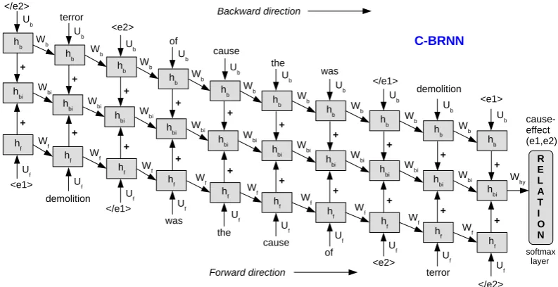
hb Wb hb hb hb hb Why R E L A T I O N Wb Wb Wb Wb <e1> demolition </e1> was the cause </e2> terror <e2> of cause the Ub Ub Ub Ub Ub Ub hb Backward direction hbi hf hbi hbi hbi hbi hbi hf hf hf hf hf Uf Uf Uf Uf Uf Uf Forward direction + + + + + + + + + + + + Wf Wf Wf Wf Wf Wbi Wbi Wbi Wbi Wbi cause-effect (e1,e2) hb Wb of was Ub hbi hf Uf + + Wf Wbi hb Wb <e2> </e1> Ub hbi hf Uf + + Wf Wbi hb Wb terror demolition Ub hbi hf Uf + + Wf Wbi hb Wb </e2> <e1> Ub hbi hf Uf + + Wf Wbi C-BRNN softmax layer
Figure 1: Connectionist Bi-directional Recurrent Neural Network (C-BRNN) (Vu et al.,2016a)
inputs. Peters et al. (2018) studied the
inter-nal states of deep bidirectiointer-nal language model to learn contextualized word representations and ob-served that the higher-level hidden states capture word semantics, while lower-level states capture syntactical aspects. Despite the possibility of visu-alizing hidden state activations and performance-based analysis, there still remains a challenge for humans to interpret hidden behavior of the“black box” networks that raised questions in the NLP community as to verify that the network behaves as expected. In this aspect, we address the cu-mulative nature of RNN with the text input and computed response to answer “how does it aggre-gate and build the semantic meaning of a sentence word by word at each time point in the sequence for each category in the data”.
Contribution: In this work, we analyze and in-terpret the cumulative nature of RNN via a
pro-posed technique named as
Layer-wIse-Semantic-Accumulation(LISA) for explaining decisions and
detecting the most likely (i.e., saliency) patterns that the network relies on while decision making.
We demonstrate (1)LISA: “How an RNN
accumu-lates or builds semantics during its sequential pro-cessing for a given text example and expected
re-sponse” (2)Example2pattern: “How the saliency
patterns look like for each category in the data ac-cording to the network in decision making”. We analyse the sensitiveness of RNNs about different inputs to check the increase or decrease in predic-tion scores. For an example sentence that is clas-sified correctly, we identify and extract a saliency
pattern (N-grams of words in order learned by the network) that contributes the most in prediction
score. Therefore, the termexample2pattern
trans-formation for each category in the data. We em-ploy two relation classification datasets: SemEval 10 Task 8 and TAC KBP Slot Filling (SF) Shared Task (ST) to explain RNN predictions via the
pro-posedLISAandexample2patterntechniques.
2 Connectionist Bi-directional RNN
We adopt the bi-directional recurrent neural net-work architecture with ranking loss, proposed by
Vu et al.(2016a). The network consists of three parts: a forward pass which processes the original
sentence word by word (Equation1); a backward
pass which processes the reversed sentence word
by word (Equation2); and a combination of both
(Equation3). The forward and backward passes
are combined by adding their hidden layers. There is also a connection to the previous combined
hid-den layer with weightWbiwith a motivation to
in-clude all intermediate hidden layers into the final
decision of the network (see Equation 3). They
named the neural architecture as ‘Connectionist
Bi-directional RNN’ (C-BRNN). Figure 1 shows
the C-BRNN architecture, where all the three parts are trained jointly.
hft =f(Uf·wt+Wf ·hft−1) (1)
hbt =f(Ub·wn−t+1+Wb·hbt+1) (2)
hbit =f(hft+hbt +Wbi·hbit−1) (3)
wherewtis the word vector of dimensiondfor
C-BRNN
<e1>
C-BRNN
<e1> demolition
C-BRNN C-BRNN C-BRNN C-BRNN C-BRNN
<e1> demolition </e1>
<e1> demolition </e1> was
<e1> demolition </e1> was the
<e1> demolition </e1> was the cause
<e1> demolition </e1> was the cause of
C-BRNN C-BRNN
<e1> demolition </e1> was the cause of <e2>
<e1> demolition </e1> was the cause of <e2> terror
0.10 0.25 0.29 0.30 0.35 0.39 0.77 0.98 1.00
C-BRNN 1.00
<e1> demolition </e1> was the cause of <e2> terror </e2> softmax
desicion layer
subsequences of sentence S1 0.10 0.20 0.30 0.40 0.50 0.60 0.70 0.80 0.90 1.00
P
re
d
ic
tio
n
pr
ob
ab
ili
ty
f
or
re
la
tio
n
in
de
x
in
s
of
tm
ax
demolition </e2>
[image:3.595.77.532.61.250.2]<e1> </e1> was the cause of <e2> terror LISA
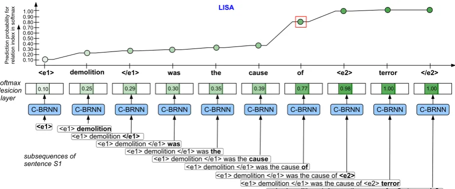
Figure 2: An illustration of Layer-wIse Semantic Accumulation (LISA) in C-BRNN, where we compute prediction score for a (known) relation type at each of the input subsequence. The highlighted indices in
the softmax layer signify one of the relation types, i.e.,cause-effect(e1, e2) in SemEval10 Task 8 dataset.
The bold signifies the last word in the subsequence. Note: Each word is represented by N-gram (N=3,
5 or 7), therefore each input subsequence is a sequence of N-grams. E.g., the word ‘of’ → ‘cause of
<e2>’ for N=3. To avoid complexity in this illustration, each word is shown as a uni-gram.
D is the hidden unit dimension. Uf ∈ Rd×D
andUb ∈ Rd×D are the weight matrices between
hidden units and input wt in forward and
back-ward networks, respectively; Wf ∈ RD×D and
Wb ∈ RD×D are the weights matrices
connect-ing hidden units in forward and backward
net-works, respectively. Wbi ∈ RD×D is the weight
matrix connecting the hidden vectors of the com-bined forward and backward network. Following
Gupta et al.(2015) during model training, we use 3-gram and 5-gram representation of each word
wtat timesteptin the word sequence, where a
3-gram forwtis obtained by concatenating the
cor-responding word embeddings, i.e.,wt−1wtwt+1.
Ranking Objective: Similar to Santos et al.
(2015) andVu et al.(2016a), we applied the
rank-ing loss function to train C-BRNN. The rankrank-ing scheme offers to maximize the distance between
the true labely+and the best competitive labelc−
given a data pointx. It is defined
as-L= log(1 + exp(γ(m+−sθ(x)y+)))
+ log(1 + exp(γ(m−+sθ(x)c−)))
(4)
wheresθ(x)y+ andsθ(x)c−being the scores for
the classes y+ andc−, respectively. The
param-eterγ controls the penalization of the prediction
errors andm+ andm are margins for the correct
and incorrect classes. FollowingVu et al.(2016a),
we setγ = 2,m+= 2.5 andm−= 0.5.
Model Training and Features: We represent each word by the concatenation of its word
em-bedding and position feature vectors. We use
word2vec (Mikolov et al., 2013) embeddings,
that are updated during model training. As po-sition features in relation classification
experi-ments, we use position indicators (PI) (Zhang and
Wang, 2015) in C-BRNN to annotate target
en-tity/nominals in the word sequence, without neces-sity to change the input vectors, while it increases the length of the input word sequences, as four
independent words, as position indicators (<e1>,
</ e1>,<e2>,</e2>) around the relation
argu-ments are introduced.
In our analysis and interpretation of recurrent neural networks, we use the trained C-BRNN
(Figure1) (Vu et al.,2016a) model.
3 LISA and Example2Pattern in RNN
There are several aspects in interpreting the
neu-ral network, for instance via (1)Data: “Which
di-mensions of the data are the most relevant for the
task” (2)Prediction orDecision: “Explain why a
certain pattern” is classified in a certain way (3) Model: “How patterns belonging to each category in the data look like according to the network”.
In this work, we focus to explain RNN via
de-cision and model aspects by finding the patterns
particu-lar decision for each category in the data and veri-fies that model behaves as expected. To do so, we propose a technique named as LISA that interprets RNN about “how it accumulates and builds mean-ingful semantics of a sentence word by word” and “how the saliency patterns look like according to the network” for each category in the data while decision making. We extract the saliency patterns
viaexample2patterntransformation.
LISA Formulation: To explain the cumula-tive nature of recurrent neural networks, we show how does it build semantic meaning of a sentence word by word belonging to a particular category in the data and compute prediction scores for the expected category on different inputs, as shown in
Figure 2. The scheme also depicts the
contribu-tion of each word in the sequence towards the final classification score (prediction probability).
At first, we compute different subsequences of word(s) for a given sequence of words (i.e.,
sentence). Consider a sequence S of words
[w1, w2, ..., wk, ..., wn] for a given sentenceS of
lengthn. We computennumber of subsequences,
where each subsequence S≤k is a subvector of
words [w1, ...wk], i.e.,S≤kconsists of words
pre-ceding and including the wordwkin the sequence
S. In context of this work, extending a quence by a word means appending the subse-quence by the next word in the sesubse-quence. Observe
that the number of subsequences,nis equal to the
total number of time steps in the C-BRNN. Next is to compute RNN prediction score for the
categoryRassociated with sentenceS. We
com-pute the score via the autoregressive conditional
P(R|S≤k,M)for each subsequenceS≤k,
as-P(R|S≤k,M) =sof tmax(Why·hbik+by) (5)
using the trained C-BRNN (Figure 1) model
M. For each k ∈ [1, n], we compute the
net-work prediction,P(R|S≤k,M)to demonstrate the
cumulative property of recurrent neural network that builds meaningful semantics of the sequence
S by extending each subsequence S≤k word by
word. The internal statehbik (attached to softmax
layer as in Figure1) is involved in decision making
for each input subsequenceS≤k with bias vector
by ∈ RC and hidden-to-softmax weights matrix
Why ∈RD×CforCcategories.
The LISAis illustrated in Figure2, where each
word in the sequence contributes to final classifi-cation score. It allows us to understand the net-work decisions via peaks in the prediction score
Algorithm 1Example2pattern Transformation
Input: sentence S, length n, category R,
thresholdτ, C-BRNNM, N-gram size N
Output:N-gram saliency patternpatt 1: forkin1tondo
2: compute N-gramk(eqn8) of words inS
3: forkin1tondo
4: computeS≤k(eqn7) of N-grams
5: computeP(R|S≤k,M)using eqn5
6: ifP(R|S≤k,M)≥τ then 7: returnpatt←S≤k[−1]
over different subsequences. The peaks signify the saliency patterns (i.e., sequence of words) that the network has learned in order to make deci-sion. For instance, the input word ‘of’ following
the subsequence ‘<e1> demolition </e1> was
the cause’ introduces a sudden increase in
pre-diction score for the relation typecause-effect(e1,
e2). It suggests that the C-BRNN collects the se-mantics layer-wise via temporally organized sub-sequences. Observe that the subsequence ‘...cause of’ is salient enough in decision making (i.e.,
pre-diction score=0.77), where the next subsequence
‘...cause of<e2>’ adds in the score to get0.98.
Example2pattern for Saliency Pattern: To further interpret RNN, we seek to identify and ex-tract the most likely input pattern (or phrases) for a given class that is discriminating enough in de-cision making. Therefore, each example input is transformed into a saliency pattern that informs us about the network learning. To do so, we first
compute N-gram for each word wt in the
sen-tence S. For instance, a 3-gram representation
of wt is given by wt−1, wt, wt+1. Therefore, an
N-gram (for N=3) sequence S of words is
rep-resented as [[wt−1, wt, wt+1]nt=1], where w0 and
wn+1 are PADDING (zero) vectors of embedding
dimension.
Following Vu et al. (2016a), we use N-grams
(e.g., tri-grams) representation for each word in
each subsequence S≤k that is input to C-BRNN
to compute P(R|S≤k), where the N-gram (N=3)
subsequenceS≤kis given by,
S≤k= [[P ADDIN G, w1, w2]1,[w1, w2, w3]2, ...,
[wt−1, wt, wt+1]t, ...,[wk−1, wk, wk+1]k]
(6)
S≤k= [tri1, tri2, ..., trit, ...trik] (7)
con-<e1 >
demolition
</e1 >was the
cause of<e2 >
terror</e2> 0
0.1 0.2 0.3 0.4 0.5 0.6 0.7 0.8 0.9 1
Prediction
Probability
cause-effect(e1, e2)
(a)LISAforS1
<e1 >
damage</e1 > caused by the <e2 > bombing< /e2> 0
0.1 0.2 0.3 0.4 0.5 0.6 0.7 0.8 0.9 1
Prediction
Probability
cause-effect(e2, e1)
(b)LISAforS2
<e1 >
courtyard<
/e1> of the<e2>castle
</e2 >
0 0.1 0.2 0.3 0.4 0.5 0.6 0.7 0.8 0.9 1
Prediction
Probability
component-whole(e1, e2)
(c)LISAforS3
<e1 >
marble</e1 >was
droppedinto the<e2
>
bowl</e2> 0
0.1 0.2 0.3 0.4 0.5 0.6 0.7 0.8 0.9 1
Prediction
Probability
entity-destination(e1, e2)
(d)LISAforS4
<e1 > car
</e1 > left the
<e2 > plant </e2 > 0 0.1 0.2 0.3 0.4 0.5 0.6 0.7 0.8 0.9 1
Prediction
Probability
entity-origin(e1, e2)
(e)LISAforS5
<e1 >
cigarettes<
/e1> by themajor<e2 >
producer< /e2> 0
0.1 0.2 0.3 0.4 0.5 0.6 0.7 0.8 0.9 1
Prediction
Probability
product-producer(e1, e2)
(f)LISAforS6
<e1 >
cigarettes<
/e1> are used by<e2> women</e2
>
0 0.1 0.2 0.3 0.4 0.5 0.6 0.7 0.8 0.9 1
Prediction
Probability
instrument-agency(e1, e2)
(g)LISAforS7
<e1 >
person</e1 > was
born in<e2> location</e2
>
0 0.1 0.2 0.3 0.4 0.5 0.6 0.7 0.8 0.9 1
Prediction
Probability
slotper:location of birth
(h)LISAforS8
<e1 >
person</e1 >
married< e2>
spouse</e2 >
0 0.1 0.2 0.3 0.4 0.5 0.6 0.7 0.8 0.9 1
Prediction
Probability
slotper:spouse
(i)LISAforS9
[image:5.595.65.524.60.697.2](j) t-SNE Visualization for training set (k) t-SNE Visualization for testing set
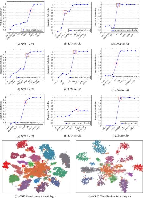
Figure 3: (a-i) Layer-wIse Semantic Accumulation (LISA) by C-BRNN for different relation types in SemEval10 Task 8 and TAC KBP Slot Filling datasets. The square in red color signifies that the relation is correctly detected with the input subsequence (enough in decision making). (j-k) t-SNE visualization
ID Relation/Slot Types Example Sentences Example2Pattern
[image:6.595.73.529.61.186.2]S1 cause-effect(e1, e2) <e1>demolition</e1>was the cause of<e2>terror</e2> cause of<e2> S2 cause-effect(e2, e1) <e1>damage</e1>caused by the<e2>bombing</e2> damage</e1>caused S3 component-whole(e1, e2) <e1>countyard</e1>of the<e2>castle</e2> </e1>of the S4 entity-destination(e1,e2) <e1>marble</e1>was dropped into the<e2>bowl</e2> dropped into the S5 entity-origin(e1, e2) <e1>car</e1>left the<e2>plant</e2> left the<e2> S6 product-produce(e1, e2) <e1>cigarettes</e1>by the major<e2>producer</e2> </e1>by the S7 instrument-agency(e1, e2) <e1>cigarettes</e1>are used by<e2>women</e2> </e1>are used S8 per:loc of birth(e1, e2) <e1>person</e1>was born in<e2>location</e2> born in<e2> S9 per:spouse(e1, e2) <e1>person</e1>married<e2>spouse</e2> </e1>married<e2>
Table 1: Example Sentences forLISAandexample2patternillustrations. The sentencesS1-S7belong to
SemEval10 Task 8 dataset andS8-S9to TAC KBP Slot Filling (SF) shared task dataset.
sists of the wordwk+1, if k6=n. To generalize for
i∈[1,bN/2c], an N-gramkof sizeNfor wordwk
in C-BRNN is given
by-N-gramk= [wk−i, ..., wk, ..., wk+i]k (8)
Algorithm1shows the transformation of an
ex-ample sentence into pattern that is salient in
deci-sion making. For a given example sentenceSwith
its lengthn and categoryR, we extract the most
salient N-gram (N=3, 5 or 7) patternpatt(the last
N-gram in the N-gram subsequenceS≤k) that
con-tributes the most in detecting the relation typeR.
The threshold parameter τ signifies the
probabil-ity of prediction for the categoryRby the model
M. For an input N-gram sequence S≤k of
sen-tenceS, we extract the last N-gram, e.g.,trikthat
detects the relationRwith prediction score above
τ. By manual inspection of patterns extracted at
different values (0.4, 0.5, 0.6, 0.7) ofτ, we found
thatτ = 0.5generates the most salient and
inter-pretable patterns. The saliency pattern detection
follows LISA as demonstrated in Figure2, except
that we use N-gram (N =3, 5 or 7) input to detect
and extract the key relationship patterns.
4 Analysis: Relation Classification
Given a sentence and two annotated nominals, the task of binary relation classification is to predict the semantic relations between the pairs of nom-inals. In most cases, the context in between the two nominals define the relationship. However,
Vu et al.(2016a) has shown that the extended con-text helps. In this work, we focus on the building semantics for a given sentence using relationship contexts between the two nominals.
We analyse RNNs for LISA and
exam-ple2pattern using two relation classification
dat-sets: (1) SemEval10 Shared Task 8 (Hendrickx
Input word sequence to C-BRNN pp
<e1> 0.10
<e1>demolition 0.25
<e1>demolition</e1> 0.29
<e1>demolition</e1>was 0.30
<e1>demolition</e1>wasthe 0.35
<e1>demolition</e1>was thecause 0.39
<e1>demolition</e1>was the causeof 0.77
<e1>demolition</e1>was the cause of<e2> 0.98
<e1>demolition</e1>was the cause of<e2>terror 1.00
<e1>demolition</e1>was the cause of<e2>terror</e2> 1.00
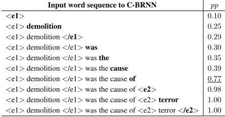
Table 2: Semantic accumulation and sensitivity
of C-BRNN over subsequences for sentence S1.
Bold indicates the last word in the subsequence.
pp: prediction probability in the softmax layer for
the relation type. The underline signifies that the
pp is sufficient enough (τ=0.50) in detecting the
relation. Saliency patterns, i.e., N-grams can be extracted from the input subsequence that leads to
a sudden peak inpp, wherepp≥τ.
et al.,2009) (2) TAC KBP Slot Filling (SF) shared task1 (Adel and Sch¨utze, 2015). We demon-strate the sensitiveness of RNN for different
sub-sequences (Figure 2), input in the same order as
in the original sentence. We explain its predic-tions (or judgments) and extract the salient rela-tionship patterns learned for each category in the two datasets.
4.1 SemEval10 Shared Task 8 dataset
The relation classification dataset of the Semantic
Evaluation 2010 (SemEval10) shared task 8 (
Hen-drickx et al.,2009) consists of 19 relations (9
di-rected relations and one artificial class Other),
8,000 training and 2,717 testing sentences. We split the training data into train (6.5k) and devel-opment (1.5k) sentences to optimize the C-BRNN
1data from the slot filler classification component of the
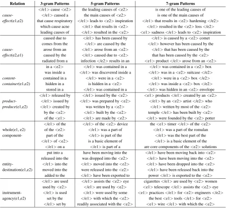
[image:6.595.306.529.242.358.2]Relation 3-gram Patterns 5-gram Patterns 7-gram Patterns </e1>cause<e2> the leading causes of<e2> is one of the leading causes of
cause- </e1>caused a the main causes of<e2> is one of the main causes of
effect(e1,e2) that cause respiratory </e1>leads to<e2>inspiration </e1>that results in<e2>hardening</e2> which cause acne </e1>that results in<e2> </e1>resulted in the<e2>loss</e2> leading causes of </e1>resulted in the<e2> <e1>sadness</e1>leads to<e2>inspiration
caused due to </e1>has been caused by </e1>is caused by a<e2>comet comes from the </e1>are caused by the </e1>however has been caused by the
cause- arose from an </e1>arose from an<e2> </e1>that has been caused by the
effect(e2,e1) caused by the </e1>caused due to<e2> that has been caused by the<e2> radiated from a infection</e2>results in an <e1>product</e1>arose from an<e2>
in a<e2> </e1>was contained in a </e1>was contained in a<e2>box was inside a </e1>was discovered inside a </e1>was in a<e2>suitcase</e2> content- contained in a </e1>were in a<e2> </e1>were in a<e2>box</e2> container(e1,e2) hidden in a is hidden in a<e2> </e1>was inside a<e2>box</e2>
stored in a </e1>was contained in a </e1>was hidden in an<e2>envelope </e1>released by </e1>issued by the<e2> <e1>products</e1>created by an<e2> product- </e1>issued by </e1>was prepared by<e2> </e1>by an<e2>artist</e2>who
produce(e1,e2) </e1>created by was written by a<e2> </e1>written by most of the<e2> by the<e2> </e1>built by the<e2> temple</e1>has been built by<e2> of the<e1> </e1>are made by<e2> </e1>were founded by the<e2>potter </e1>of the </e1>of the<e2>device the<e1>timer</e1>of the<e2> whole(e1, e2) of the<e2> </e1>was a part of </e1>was a part of the romulan component- part of the </e1>is part of the </e1>was the best part of the
</e1>of<e2> is a basic element of </e1>is a basic element of the </e1>on a </e1>is part of a are core components of the<e2>solutions
put into a have been moving into the </e1>have been moving back into<e2> released into the was dropped into the<e2> </e1>have been moving into the<e2> entity- </e1>into the </e1>moved into the<e2> </e1>have been dropped into the<e2> destination(e1,e2) moved into the were released into the<e2> </e1>have been released back into the
added to the </e1>have been exported to power</e1>is exported to the<e2> </e1>are used </e1>assists the<e2>eye cigarettes</e1>are used by<e2>women
used by<e2> </e1>are used by<e2> <e1>telescope</e1>assists the<e2>eye instrument- </e1>is used </e1>were used by some <e1>practices</e1>for<e2>engineers</e2> agency(e1,e2) set by the </e1>with which the<e2> the best<e1>tools</e1>for<e2>
[image:7.595.74.524.61.476.2]</e1>set by readily associated with the<e2> <e1>wire</e1>with which the<e2>
Table 3: SemEval10 Task 8 dataset: N-Gram (3, 5 and 7) saliency patterns extracted for different relation types by C-BRNN with PI
network. For instance, an example sentence with relation label is given
by-The <e1> demolition </e1> was
the cause of <e2> terror </e2>
and communal divide is just a way
of not letting truth prevail. →
cause-effect(e1,e2)
The terms demolition and terror are
the relation arguments or nominals, where the
phrasewas the cause ofis the relationship
context between the two arguments. Table 1
shows the examples sentences (shortened to ar-gument1+relationship context+argument2) drawn from the development and test sets that we em-ployed to analyse the C-BRNN for semantic accu-mulation in our experiments. We use the similar
experimental setup asVu et al.(2016a).
LISA Analysis: As discussed in Section 3, we
interpret C-BRNN by explaining its predictions via the semantic accumulation over the
subse-quencesS≤k (Figure2) for each sentenceS. We
select the example sentencesS1-S7(Table 1) for
which the network predicts the correct relation type with high scores. For an example sentence
S1, Table2illustrates how different subsequences
are input to C-BRNN in order to compute
predic-tion scoresppin the softmax layer for the relation
cause-effect(e1, e2). We use tri-gram
(section3) word representation for each word for
the examplesS1-S7.
Figures 3a, 3b, 3c, 3d 3e, 3f and 3g
demon-strate the cumulative nature and sensitiveness of
RNN via prediction probability (pp) about
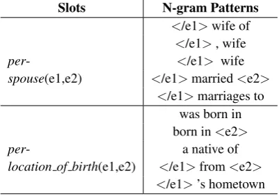
Slots N-gram Patterns
</e1>wife of
</e1>, wife
per- </e1> wife
spouse(e1,e2) </e1>married<e2>
</e1>marriages to was born in born in<e2>
per- a native of
location of birth(e1,e2) </e1>from<e2>
[image:8.595.81.282.63.204.2]</e1>’s hometown
Table 4: TAC KBP SF dataset: Tri-gram saliency
patterns extracted for slotsper:spouse(e1, e2) and
per:location of birth(e1,e2)
instance in Figure 3a and Table 2, the C-BRNN
builds meaning of the sentenceS1word by word,
where a sudden increase in pp is observed when
the input subsequence <e1> demolition
</e1> was the causeis extended with the
next term ofin the word sequenceS. Note that
the relationship context between the arguments
demolition andterroris sufficient enough
in detecting the relationship type. Interestingly,
we also observe that the prepositions (such asof,
by,into, etc.) in combination with verbs are key
features in building the meaningful semantics.
Saliency Patterns via example2pattern Trans-formation: Following the discussion in Section
3 and Algorithm 1, we transform each correctly
identified example into pattern by extracting the most likely N-gram in the input subsequence(s).
In each of the Figures3a,3b,3c,3d 3e,3fand3g,
the square box in red color signifies that the
rela-tion type is correctly identified (whenτ = 0.5) at
this particular subsequence input (without the re-maining context in the sentence). We extract the last N-gram of such a subsequence.
Table1shows theexample2pattern
transforma-tions for sentencesS1-S7in SemEval10 dataset,
derived from Figures3a-3g, respectively with N=3
(in the N-grams). Similarly, we extract the salient
patterns (3-gram, 5-gram and 7-gram) (Table 3)
for different relationships. We also observe that
the relation typescontent-container(e1,
e2) and instrument-agency(e1,
e2) are mostly defined by smaller
rela-tionship contexts (e.g, 3-gram), however
entity-destination(e1,e2) by larger
contexts (7-gram).
4.2 TAC KBP Slot Filling dataset
We investigate another dataset from TAC KBP
Slot Filling (SF) shared task (Surdeanu, 2013),
where we use the relation classification dataset by
Adel et al.(2016) in the context of slot filling. We
have selected the two slots: per:loc of birth and
per:spouseout of 24 types.
LISA Analysis: Following Section4.1, we
anal-yse the C-BRNN for LISA using sentences S8
andS9(Table1). Figures3h and3idemonstrate
the cumulative nature of recurrent neural network,
where we observe that the salient patternsborn
in <e2> and </e1> married e2 lead to
correct decision making for S8 and S9,
respec-tively. Interestingly forS8, we see a decrease in
prediction score from 0.59 to 0.52 on including
terms in the subsequence, following the termin.
Saliency Patterns via example2pattern
Trans-formation: Following Section 3and Algorithm1,
we demonstrate the example2pattern
transforma-tion of sentences S8 and S9 in Table 1 with
tir-grams. In addition, Table 4 shows the tri-gram
salient patterns extracted for the two slots.
5 Visualizing Latent Semantics
In this section, we attempt to visualize the hidden state of each test (and train) example that has ac-cumulated (or built) the meaningful semantics dur-ing sequential processdur-ing in C-BRNN. To do this,
we compute the last hidden vectorhbiof the
com-bined network (e.g., hbi attached to the softmax
layer in Figure1) for each test (and train)
exam-ple and visualize (Figure3k and3j) using t-SNE
(Maaten and Hinton,2008). Each color represents a relation-type. Observe the distinctive clusters of accumulated semantics in hidden states for each category in the data (SemEval10 Task 8).
6 Conclusion and Future Work
We have demonstrated the cumulative nature of recurrent neural networks via sensitivity analysis
over different inputs, i.e.,LISAto understand how
they build meaningful semantics and explain pre-dictions for each category in the data. We have also detected a salient pattern in each of the
exam-ple sentences, i.e., example2pattern
transforma-tion that the network learns in decision making.
We extract the salient patterns for different cate-gories in two relation classification datasets.
the salient patterns. One could also investigate visualizing the dimensions of hidden states (acti-vation maximization) and word embedding vec-tors with the network decisions over time. We
forsee to applyLISAandexample2patternon
dif-ferent tasks such as document categorization,
sen-timent analysis, language modeling, etc.
An-other interesting direction would be to analyze the bag-of-word neural topic models such as
Doc-NADE (Larochelle and Lauly, 2012) and
iDoc-NADE (Gupta et al.,2018b) to interpret their
se-mantic accumulation during autoregressive com-putations in building document representation(s). We extract the saliency patterns for each cate-gory in the data that can be effectively used in instantiating pattern-based information extraction
systems, such as bootstrapping entity (Gupta and
Manning, 2014) and relation extractors (Gupta et al.,2018e).
Acknowledgments
We thank Heike Adel for providing us with the TAC KBP dataset used in our
experi-ments. We express appreciation for our
col-leagues Bernt Andrassy, Florian Buettner, Ulli Waltinger, Mark Buckley, Stefan Langer, Subbu Rajaram, Yatin Chaudhary, and anonymous re-viewers for their in-depth review comments. This research was supported by Bundeswirtschaftsmin-isterium (bmwi.de), grant 01MD15010A (Smart Data Web) at Siemens AG- CT Machine Intelli-gence, Munich Germany.
References
Heike Adel, Benjamin Roth, and Hinrich Sch¨utze. 2016. Comparing convolutional neural networks to traditional models for slot filling. InProceedings of the 2016 Conference of the North American Chap-ter of the Association for Computational
Linguis-tics: Human Language Technologies, pages 828–
838. Association for Computational Linguistics.
Heike Adel and Hinrich Sch¨utze. 2015. Cis at tac cold start 2015: Neural networks and coreference resolu-tion for slot filling. Proc. TAC2015.
Sebastian Bach, Alexander Binder, Gr´egoire Mon-tavon, Frederick Klauschen, Klaus-Robert M¨uller, and Wojciech Samek. 2015. On pixel-wise explana-tions for non-linear classifier decisions by layer-wise relevance propagation. PloS one, 10(7):e0130140.
David Baehrens, Timon Schroeter, Stefan Harmel-ing, Motoaki Kawanabe, Katja Hansen, and Klaus-Robert M ˜Aˇzller. 2010. How to explain individual
classification decisions. Journal of Machine
Learn-ing Research, 11(Jun):1803–1831.
Dzmitry Bahdanau, Kyunghyun Cho, and Yoshua Ben-gio. 2014. Neural machine translation by jointly learning to align and translate. arXiv preprint
arXiv:1409.0473.
Alexey Dosovitskiy and Thomas Brox. 2016. Inverting visual representations with convolutional networks.
In Proceedings of the IEEE Conference on
Com-puter Vision and Pattern Recognition, pages 4829–
4837.
Jeffrey L Elman. 1990. Finding structure in time.
Cog-nitive science, 14(2):179–211.
Dumitru Erhan, Yoshua Bengio, Aaron Courville, and Pascal Vincent. 2009. Visualizing higher-layer fea-tures of a deep network. University of Montreal, 1341(3):1.
Ian J Goodfellow, Jonathon Shlens, and Christian Szegedy. 2014. Explaining and harnessing adver-sarial examples. arXiv preprint arXiv:1412.6572.
Pankaj Gupta, Bernt Andrassy, and Hinrich Sch¨utze. 2018a. Replicated siamese lstm in ticketing sys-tem for similarity learning and retrieval in asymmet-ric texts. In Proceedings of the Workshop on Se-mantic Deep Learning (SemDeep-3) in the 27th In-ternational Conference on Computational
Linguis-tics (COLING2018). The COLING 2018 organizing
committee.
Pankaj Gupta, Florian Buettner, and Hinrich Sch¨utze. 2018b. Document informed neural autoregres-sive topic models. Researchgate preprint doi: 10.13140/RG.2.2.12322.73925.
Pankaj Gupta, Subburam Rajaram, Thomas Runk-ler, Hinrich Sch¨utze, and Bernt Andrassy. 2018c. Neural relation extraction within and across sen-tence boundaries. Researchgate preprint doi: 10.13140/RG.2.2.16517.04327.
Pankaj Gupta, Subburam Rajaram, Hinrich Sch¨utze, and Bernt Andrassy. 2018d. Deep temporal-recurrent-replicated-softmax for topical trends over time. In Proceedings of the 2018 Conference of the North American Chapter of the Association for Computational Linguistics: Human Language
Technologies, Volume 1 (Long Papers), volume 1,
pages 1079–1089, New Orleans, USA. Association of Computational Linguistics.
Pankaj Gupta, Benjamin Roth, and Hinrich Sch¨utze. 2018e. Joint bootstrapping machines for high confi-dence relation extraction. InProceedings of the 16th Annual Conference of the North American Chap-ter of the Association for Computational
Linguis-tics: Human Language Technologies (Long Papers),
Pankaj Gupta, Thomas Runkler, Heike Adel, Bernt Andrassy, Hans-Georg Zimmermann, and Hinrich Sch¨utze. 2015. Deep learning methods for the ex-traction of relations in natural language text. Tech-nical report, TechTech-nical University of Munich, Ger-many.
Pankaj Gupta, Hinrich Sch¨utze, and Bernt Andrassy. 2016. Table filling multi-task recurrent neural net-work for joint entity and relation extraction. In Pro-ceedings of COLING 2016, the 26th International Conference on Computational Linguistics:
Techni-cal Papers, pages 2537–2547. The COLING 2016
Organizing Committee.
Sonal Gupta and Christopher Manning. 2014. Spied: Stanford pattern based information extraction and diagnostics. InProceedings of the Workshop on teractive Language Learning, Visualization, and
In-terfaces, pages 38–44.
Iris Hendrickx, Su Nam Kim, Zornitsa Kozareva, Preslav Nakov, Diarmuid ´O S´eaghdha, Sebastian Pad´o, Marco Pennacchiotti, Lorenza Romano, and Stan Szpakowicz. 2009. Semeval-2010 task 8: Multi-way classification of semantic relations be-tween pairs of nominals. In Proceedings of
the Workshop on Semantic Evaluations: Recent
Achievements and Future Directions, pages 94–99.
Association for Computational Linguistics.
Geoffrey E Hinton. 2012. A practical guide to training restricted boltzmann machines. InNeural networks:
Tricks of the trade, pages 599–619. Springer.
Sepp Hochreiter and J¨urgen Schmidhuber. 1997. Long short-term memory. Neural computation, 9(8):1735–1780.
Guillaume Lample, Miguel Ballesteros, Sandeep Sub-ramanian, Kazuya Kawakami, and Chris Dyer. 2016. Neural architectures for named entity recognition.
InProceedings of the 2016 Conference of the North
American Chapter of the Association for
Computa-tional Linguistics: Human Language Technologies,
pages 260–270. Association for Computational Lin-guistics.
Hugo Larochelle and Stanislas Lauly. 2012. A neural autoregressive topic model. In F. Pereira, C. J. C. Burges, L. Bottou, and K. Q. Weinberger, editors,
Advances in Neural Information Processing Systems 25, pages 2708–2716. Curran Associates, Inc.
Jiwei Li, Xinlei Chen, Eduard Hovy, and Dan Jurafsky. 2016. Visualizing and understanding neural models in nlp. In Proceedings of the 2016 Conference of the North American Chapter of the Association for Computational Linguistics: Human Language
Tech-nologies, pages 681–691. Association for
Computa-tional Linguistics.
Xuezhe Ma and Eduard Hovy. 2016. End-to-end se-quence labeling via bi-directional lstm-cnns-crf. In
Proceedings of the 54th Annual Meeting of the As-sociation for Computational Linguistics (Volume 1:
Long Papers), pages 1064–1074. Association for
Computational Linguistics.
Laurens van der Maaten and Geoffrey Hinton. 2008. Visualizing data using t-sne. Journal of machine
learning research, 9(Nov):2579–2605.
Gr´egoire Mesnil, Yann Dauphin, Kaisheng Yao, Yoshua Bengio, Li Deng, Dilek Hakkani-Tur, Xi-aodong He, Larry Heck, Gokhan Tur, Dong Yu, et al. 2015. Using recurrent neural networks for slot fill-ing in spoken language understandfill-ing. IEEE/ACM Transactions on Audio, Speech, and Language
Pro-cessing, 23(3):530–539.
Tomas Mikolov, Kai Chen, Greg Corrado, and Jeffrey Dean. 2013. Efficient estimation of word represen-tations in vector space. InProceedings of the
Work-shop at ICLR.
Tom´aˇs Mikolov, Martin Karafi´at, Luk´aˇs Burget, Jan ˇ
Cernock`y, and Sanjeev Khudanpur. 2010. Recur-rent neural network based language model. In
Eleventh Annual Conference of the International
Speech Communication Association.
Yao Ming, Shaozu Cao, Ruixiang Zhang, Zhen Li, Yuanzhe Chen, Yangqiu Song, and Huamin Qu. 2017. Understanding hidden memories of recurrent neural networks. arXiv preprint arXiv:1710.10777.
Makoto Miwa and Mohit Bansal. 2016. End-to-end re-lation extraction using lstms on sequences and tree structures. InProceedings of the 54th Annual Meet-ing of the Association for Computational LMeet-inguistics
(Volume 1: Long Papers), pages 1105–1116.
Asso-ciation for Computational Linguistics.
Gr´egoire Montavon, Wojciech Samek, and Klaus-Robert M¨uller. 2017. Methods for interpreting and understanding deep neural networks. Digital Signal
Processing.
Jonas Mueller and Aditya Thyagarajan. 2016. Siamese recurrent architectures for learning sentence similar-ity. InAAAI, volume 16, pages 2786–2792.
Anh Nguyen, Alexey Dosovitskiy, Jason Yosinski, Thomas Brox, and Jeff Clune. 2016. Synthesizing the preferred inputs for neurons in neural networks via deep generator networks. InAdvances in Neural
Information Processing Systems, pages 3387–3395.
Matthew Peters, Mark Neumann, Mohit Iyyer, Matt Gardner, Christopher Clark, Kenton Lee, and Luke Zettlemoyer. 2018. Deep contextualized word repre-sentations. InProceedings of the 2018 Conference of the North American Chapter of the Association for Computational Linguistics: Human Language
Technologies, Volume 1 (Long Papers), pages 2227–
2237. Association for Computational Linguistics.
Karen Simonyan, Andrea Vedaldi, and Andrew Zisser-man. 2013. Deep inside convolutional networks: Vi-sualising image classification models and saliency maps. arXiv preprint arXiv:1312.6034.
Mihai Surdeanu. 2013. Overview of the tac2013 knowledge base population evaluation: English slot filling and temporal slot filling. InTAC.
Duyu Tang, Bing Qin, and Ting Liu. 2015. Docu-ment modeling with gated recurrent neural network for sentiment classification. In Proceedings of the 2015 Conference on Empirical Methods in Natural
Language Processing, pages 1422–1432.
Associa-tion for ComputaAssocia-tional Linguistics.
Zhiyuan Tang, Ying Shi, Dong Wang, Yang Feng, and Shiyue Zhang. 2017. Memory visualization for gated recurrent neural networks in speech recogni-tion. In Acoustics, Speech and Signal Processing
(ICASSP), 2017 IEEE International Conference on,
pages 2736–2740. IEEE.
Ngoc Thang Vu, Heike Adel, Pankaj Gupta, and Hin-rich Sch¨utze. 2016a. Combining recurrent and con-volutional neural networks for relation classifica-tion. InProceedings of the North American Chap-ter of the Association for Computational
Linguis-tics: Human Language Technologies, pages 534–
539, San Diego, California USA. Association for Computational Linguistics.
Ngoc Thang Vu, Pankaj Gupta, Heike Adel, and Hinrich Sch¨utze. 2016b. Bi-directional recurrent neural network with ranking loss for spoken lan-guage understanding. InProceedings of the
Acous-tics, Speech and Signal Processing (ICASSP), pages
6060–6064, Shanghai, China. IEEE.
Yequan Wang, Minlie Huang, xiaoyan zhu, and Li Zhao. 2016. Attention-based lstm for aspect-level sentiment classification. InProceedings of the 2016 Conference on Empirical Methods in Natural
Lan-guage Processing, pages 606–615. Association for
Computational Linguistics.
Matthew D Zeiler and Rob Fergus. 2014. Visualizing and understanding convolutional networks. In
Eu-ropean conference on computer vision, pages 818–
833. Springer.