Storing the Web in Memory: Space Efficient Language Models with
Constant Time Retrieval
David Guthrie
Computer Science Department University of Sheffield [email protected]
Mark Hepple
Computer Science Department University of Sheffield [email protected]
Abstract
We present three novel methods of compactly storing very large n-gram language models. These methods use substantially less space than all known approaches and allown-gram probabilities or counts to be retrieved in con-stant time, at speeds comparable to modern language modeling toolkits. Our basic ap-proach generates anexplicit minimal perfect hash function, that maps all n-grams in a model to distinct integers to enable storage of associated values. Extensions of this approach exploit distributional characteristics ofn-gram data to reduce storage costs, including variable length coding of values and the use oftiered structures that partition the data for more effi-cient storage. We apply our approach to stor-ing the full Google Web1Tn-gram set and all 1-to-5 grams of the Gigaword newswire cor-pus. For the 1.5 billionn-grams of Gigaword, for example, we can store full count informa-tion at a cost of 1.66 bytes pern-gram (around 30% of the cost when using the current state-of-the-art approach), or quantized counts for 1.41 bytes pern-gram. For applications that are tolerant of a certain class of relatively in-nocuous errors (where unseen n-grams may be accepted as raren-grams), we can reduce the latter cost to below 1 byte pern-gram.
1 Introduction
The availability of very large text collections, such as the Gigaword corpus of newswire (Graff, 2003), and the Google Web1T 1-5gram corpus (Brants and Franz, 2006), have made it possible to build
mod-els incorporating counts of billions ofn-grams. The
storage of these language models, however, presents
serious problems, given both their size and the need to provide rapid access. A prevalent approach for language model storage is the use of compact trie structures, but these structures do not scale well and require space proportional to both to the number
of n-grams and the vocabulary size. Recent
ad-vances (Talbot and Brants, 2008; Talbot and Os-borne, 2007b) involve the development of Bloom fil-ter based models, which allow a considerable reduc-tion in the space required to store a model, at the cost of allowing some limited extent of false positives when the model is queried with previously unseen n-grams. The aim is to achieve sufficiently compact representation that even very large language models can be stored totally within memory, avoiding the latencies of disk access. These Bloom filter based models exploit the idea that it is not actually
neces-sary tostore then-grams of the model, as long as,
when queried with ann-gram, the model returns the
correct count or probability for it. These techniques allow the storage of language models that no longer depend on the size of the vocabulary, but only on the
number ofn-grams.
In this paper we give three different models for the efficient storage of language models. The first structure makes use of an explicit perfect hash
func-tion that is minimal in that it maps n keys to
in-tegers in the range 1 to n. We show that by
us-ing a minimal perfect hash function and exploit-ing the distributional characteristics of the data we
producen-gram models that use less space than all
know approaches with no reduction in speed. Our two further models achieve even more compact stor-age while maintaining constant time access by
us-ing variable length codus-ing to compress then-grams
values and by using tiered hash structures to
tion the data into subsets requiring different amounts of storage. This combination of techniques allows
us, for example, to represent thefullcount
informa-tion of the Google Web1T corpus (Brants and Franz, 2006) (where count values range up to 95 billion) at
a cost of just 2.47 bytes per n-gram (assuming
8-bit fingerprints, to exclude false positives) and just
1.41 bytes per n-gram if we use 8-bit quantization
of counts. These costs are 36% and 57% respec-tively of the space required by the Bloomier Filter approach of Talbot and Brants (2008). For the Gi-gaword dataset, we can store full count information
at a cost of only 1.66 bytes per n-gram. We
re-port empirical results showing that our approach al-lows a look-up rate which is comparable to existing modern language modeling toolkits, and much faster than a competitor approach for space-efficient
stor-age. Finally, we propose the use ofvariable length
fingerprintingfor use in contexts which can tolerate
a higher rate of ‘less damaging’ errors. This move allows, for example, the cost of storing a quantized
model to be reduced to 1 byte pern-gram or less.
2 Related Work
A range of lossy methods have been proposed, to
reduce the storage requirements of LMs by discard-ing information. Methods include the use of entropy pruning techniques (Stolcke, 1998) or clustering (Je-linek et al., 1990; Goodman and Gao, 2000) to
re-duce the number of n-grams that must be stored.
A key method is quantization (Whittaker and Raj,
2001), which reduces the value information stored
withn-grams to a limited set ofdiscretealternatives.
It works by grouping together the values
(probabil-ities or counts) associated with n-grams into
clus-ters, and replacing the value to be stored for each n-gram with a code identifying its value’s cluster.
For a scheme with n clusters, codes require log2n
bits. A common case is 8-bit quantization,
allow-ing up to 256 distinct ‘quantum’ values.
Differ-ent methods of dividing the range of values into
clusters have been used, e.g. Whittaker and Raj
(2001) used the Lloyd-Max algorithm, whilst Fed-erico and Bertoldi (2006) use the simpler Binning method to quantize probabilities, and show that the LMs so produced out-perform those produced us-ing the Lloyd-Max method on a phrase-based
ma-chine translation task. Binning partitions the range of values into regions that are uniformly populated, i.e. producing clusters that contain the same num-ber of unique values. Functionality to perform uni-form quantization of this kind is provided as part of various LM toolkits, such as IRSTLM. Some of the empirical storage results reported later in the paper
relate to LMs recordingn-gramcountvalues which
have been quantized using this uniform binning ap-proach. In the rest of this section, we turn to look
at some of the approaches used forstoringlanguage
models, irrespective of whether lossy methods are first applied to reduce the size of the model.
2.1 Language model storage using Trie
structures
A widely used approach for storing language
mod-els employs thetriedata structure (Fredkin, 1960),
which compactly represents sequences in the form
of a prefix tree, where each step down from the
root of the tree adds a new element to the sequence represented by the nodes seen so far. Where two sequences share a prefix, that common prefix is jointly represented by a single node within the trie. For language modeling purposes, the steps through
the trie correspond to words of the vocabulary,
al-though these are in practice usually represented by 24 or 32 bit integers (that have been uniquely as-signed to each word). Nodes in the trie
correspond-ing to complete n-grams can store other
informa-tion, e.g. a probability or count value. Most mod-ern language modeling toolkits employ some ver-sion of a trie structure for storage, including SRILM (Stolcke, 2002), CMU toolkit (Clarkson and Rosen-feld, 1997), MITLM (Hsu and Glass, 2008), and IRSTLM (Federico and Cettolo, 2007) and imple-mentations exist which are very compact (Germann et al., 2009). An advantage of this structure is that it
allows the storedn-grams to be enumerated.
approach present further obstacles to rapid access.
2.2 Bloom Filter Based Language Models
Recent randomized language models (Talbot and Osborne, 2007b; Talbot and Osborne, 2007a; bot and Brants, 2008; Talbot and Talbot, 2008; Tal-bot, 2009) make use of Bloom filter like structures
to map n-grams to their associated probabilities or
counts. These methods store language models in
relatively little space by not actually keeping the
n-gram key in the structure and by allowing a small probability of returning a false positive, i.e. so that
for an n-gram that is not in the model, there is a
small risk that the model will return some random
probability instead of correctly reporting that the
n-gram was not found. These structures do not allow
enumeration over then-grams in the model, but for
many applications this is not a requirement and their space advantages make them extremely attractive. Two major approaches have been used for storing language models: Bloom Filters and Bloomier Fil-ters. We give an overview of both in what follows.
2.2.1 Bloom Filters
A Bloom filter (Bloom, 1970) is a compact data structure for membership queries, i.e. queries of the form “Is this key in the Set?”. This is a weaker struc-ture than a dictionary or hash table which also asso-ciates a value with a key. Bloom filters use well be-low the information theoretic be-lower bound of space required to actually store the keys and can answer queries in O(1) time. Bloom filters achieve this feat by allowing a small probability of returning a false
positive. A Bloom filter stores a setSofnelements
in a bit arrayB of sizem. InitiallyB is set to
con-tain all zeros. To store an itemx from S inB we
compute k random independent hash functions on
xthat each return a value in the range[0. . m−1].
These values serve as indices to the bit arrayB and
the bits at those positions are set to 1. We do this
for all elements inS, storing to the same bit array.
Elements may hash to an index inBthat has already
been set to 1 and in this case we can think of these elements as “sharing” this bit. To test whether set S
contains a keyw, we run ourkhash functions onw
and check if all those locations inB are set to 1. If
w∈S then the bloom filter will always declare that
wbelongs toS, but ifx /∈Sthen the filter can only
say with high probability thatwis not inS. This
er-ror rate depends on the number ofkhash functions
and the ratio ofm/n. For instance withk = 3hash
functions and a bit array of sizem = 20n, we can
expect to get a false positive rate of 0.0027.
Talbot and Osborne (2007b) and Talbot and Os-borne (2007a) adapt Bloom filters to the requirement
of storing values forn-grams by concatenating the
key (n-gram) and value to form a single item that is inserted into the filter. Given a quantization scheme
allowing values in the range [1. . V], a quantized
valuevis stored by inserting into the filter all
pair-ings of then-gram with values from 1 up tov. To
re-trieve the value for a given key, we serially probe the filter for pairings of the key with each value from 1 upwards, until the filter returns false. The last value found paired with the key in the filter is the value re-turned. Talbot and Osborne use a simple logarithmic quantization of counts that produce limited quan-tized value ranges, where most items will have val-ues that are low in the range, so that the serial look-up process will require quite a low number of steps on average. For alternative quantization schemes that involve greater value ranges (e.g. the 256 values
of a uniform 8-bit scheme) and/or distributen-grams
more evenly across the quantized values, the average number of look-up steps required will be higher and
hence the speed of access per n-gram accordingly
lower. In that case also, the requirement of
insert-ingn-grams more than once in the filter (i.e. with
values from 1 up to the actual valuevbeing stored)
could substantially reduce the space efficiency of the method, especially if low false positive rates are
re-quired, e.g. the case k = 3, m = 20nproduces a
false positive rate of 0.0027, as noted above, but in a situation where 3 key-value items were being stored
pern-gram on average, this error rate would in fact
require a storage cost of 60 bits per originaln-gram.
2.2.2 Bloomier Filters
More recently, Talbot and Brants (2008) have pro-posed an approach to storing large language
mod-els which is based on theBloomier Filtertechnique
of Chazelle et al. (2004). Bloomier Filters gener-alize the Bloom Filter to allow values for keys to be stored in the filter. To test whether a given key is present in a populated Bloomier filter, we apply
indices for retrieving the data stored at klocations within the filter, similarly to look-up in a Bloom fil-ter. In this case, however, the data retrieved from the
filter consists ofkbit vectors, which are combined
with a fingerprint of the key, usingbitwise XOR, to
return the stored value. The risk of false positives is managed by making incorporating a fingerprint of
then-gram, and by making bit vectors longer than
the minimum length required to store values. These
additionalerror bitshave a fairly predictable impact
on error rates, i.e. witheerror bits, we anticipate the
probability of falsely construing an unseenn-gram
as being stored in the filter to be 2−e. The
algo-rithm required to correctly populate the Bloomier fil-ter with stored data is complicated, and we shall not
consider its details here. Nevertheless, when usingv
bits to represent values andebits for error detection,
this approach allows a language model to be stored at a cost of is1.23·(v+e)bits pern-gram.
3 Single Minimal Perfect Hash Ranking Approach
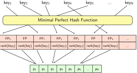
We first describe our basic structure we call Single Minimal Perfect Hash Rank (S-MPHR) that is more compact than that of Talbot and Brants (2008) while still keeping a constant look up time. In the next two sections we describe variations on this model to further reduce the space required while maintaining a constant look up time. The S-MPHR structure can be divided into 3 parts as shown in Figure 1: Stage 1 is a minimal perfect hash function; Stage 2 is a fingerprint and rank array; and Stage 3 is a unique value array. We discuss each stage in turn.
FP5 FP FP1 FP3 FP2 FP FP4 ...
key1 key2 key3 key4 key5 ... keyN
Minimal Perfect Hash Function
Array of K distinct probability values / frequency counts
p1 p2 p3 p4 p5 p6 ... pK
[image:4.612.73.300.523.644.2]rank(key5) rank(key) rank(key1) rank(key3) rank(key2) rank(key) rank(key4) ...
Figure 1: The Single MPHR structure
3.1 Minimal Perfect Hash Function
The first part of the structure is a minimal perfect
hash function that maps everyn-gram in the training
data to a distinct integer in the range 0 to N −1,
whereN is the total number ofn-grams to store. We
use these integers as indices into the array of Stage 2 of our structure.
We use theHash, displace, and compress (CHD)
(Belazzougui et al., 2009) algorithm to generate a
minimal perfect hash function that requires2.07bits
per key and hasO(1)access. The algorithm works
as follows. Given a set S that contains N = |S|
keys (in our casen-grams) that we wish to map to
integers in the range0toN −1, so that every key
maps to a distinct integer (no collisions).
The first step is to use a hash function g(x), to
map every key to a bucket B in the range 0 to r.
(For this step we use a simple hash function like the one used for generating fingerprints in the pervious section.)
Bi ={x∈S|g(x) =i}0≤i≤r
The functiong(x)is not perfect so several keys can
map to the same bucket. Here we chooser ≤ N,
so that the number of buckets is less than or equal to the number of keys (to achieve 2.07 bits per key
we user = N5, so that the average bucket size is 5).
The buckets are then sorted into descending order
according to the number of keys in each bucket|Bi|.
For the next step, a bit array,T, of sizeN is
ini-tialized to contain all zerosT[0. . . N −1]. This bit array is used during construction to keep track of
which integers in the range0toN −1the minimal
perfect hash has already mapped keys to. Next we must assume we have access to a family of random and independent hash functions h1, h2, h3, . . . that
can be accessed using an integer index. In practice it sufficient to use functions that behave similarly to fully random independent hash functions and Belaz-zougui et al. (2009) demonstrate how such functions can be generated easily by combining two simple hash functions.
Next is the “displacement” step. For each bucket, in the sorted order from largest to smallest, they search for a random hash function that maps all
ele-ments of the bucket to values inT that are currently
positions inT are set to1. So, for each bucketBi,
it is necessary to iteratively try hash functions, h`
for` = 1,2,3, . . .to hash every element ofBito a
distinct indexjinT that contains a zero.
{h`(x)|x∈Bi} ∩ {j|T[j] = 1}=∅
where the size of{h`(x)|x∈Bi}is equal to the size
ofBi. When such a hash function is found we need
only to store the index,`, of the successful function
in an arrayσand setT[j] = 1for all positionsjthat
h`hashed to. Notice that the reason the largest
buck-ets are handled first is because they have the most el-ements to displace and this is easier when the array
T contains more empty positions (zeros).
The final step in the algorithm is to compress theσ
array (which has length equal to the number of
buck-ets|B|), retainingO(1)access. This compression is
achieved using simple variable length encoding with an index array (Fredriksson and Nikitin, 2007).
3.2 Fingerprint and Rank Array
The hash function used in Stage 1 is perfect, so it
is guaranteed to return unique integers for seen
n-grams, but our hash function will also return
inte-ger values in the range0toN −1forn-grams that
have not been seen before (were not used to build the hash function). To reduce the probability of these
unseen n-grams giving false positives results from
our model we store a fingerprint of eachn-gram in
Stage 2 of our structure that can be compared against
the fingerprints of unseen n-grams when queried.
If these fingerprints of the queriedn-gram and the
stored n-gram do not match then the model will
correctly report that the n-gram has not been seen
before. The size of this fingerprint determines the rate of false positives. Assuming that the finger-print is generated by a random hash function, and
that the returned integer of anunseen key from the
MPH function is also random, expected false posi-tive rate for the model is the same as the probabil-ity of two keys randomly hashing to the same value,
1
2m, where m is the number of bits of the
finger-print. The fingerprint can be generated using any suitably random hashing algorithm. We use Austin
Appleby’s Murmurhash21implementation to
finger-print eachn-gram and then store them highest
or-der bits. Stage 2 of the MPHR structure also stores
1http://murmurhash.googlepages.com/
arankfor everyn-gram along with the fingerprint.
This rank is an index into the array of Stage 3 of our structure that holds the unique values associated
with anyn-gram.
3.3 Unique Value Array
We describe our storage of the values associated
withn-grams in our model assuming we are storing
frequency “counts” ofn-grams, but it applies also to
storing quantized probabilities. For every n-gram,
we store the ‘rank’ of the frequency countr(key),
(r(key) ∈ [0...R−1]) and use a separate array in
Stage 3 to store the frequency count value. This is similar to quantization in that it reduces the num-ber of bits required for storage, but unlike quanti-zation it does not require a loss of any information.
This was motivated by the sparsity of n-gram
fre-quency counts in corpora in the sense that if we take
the lowest n-gram frequency count and the
high-est n-gram frequency count then most of the
inte-gers in that range do not occur as a frequency count
of any n-grams in the corpus. For example in the
Google Web1T data, there are 3.8 billion unique
n-grams with frequency counts ranging from 40 to 95
Billion yet these n-grams only have 770 thousand
distinct frequency counts (see Table 2). Because we only store the frequency rank, to keep the
pre-cise frequency information we need onlydlog2Ke
bits pern-gram, whereK is the number of distinct
frequency counts. To keep all information in the
Google Web1T data we need onlydlog2771058e=
20 bits per n-gram. Rather than the bits needed
to store the maximum frequency count associated
with ann-gram,dlog2maxcounte, which for Google
Web1T would bedlog295119665584e= 37bits per
n-gram.
unique maximumn-gram unique
n-grams frequency count counts 1gm 1,585,620 71,363,822 16,896 2gm 55,809,822 9,319,466 20,237 3gm 250,928,598 829,366 12,425 4gm 493,134,812 231,973 6,838 5gm 646,071,143 86,943 4,201 Total 1,447,529,995 71,363,822 60,487
unique maximumn-gram unique
[image:6.612.314.546.53.201.2]n-grams frequency count counts 1gm 13,588,391 95,119,665,584 238,592 2gm 314,843,401 8,418,225,326 504,087 3gm 977,069,902 6,793,090,938 408,528 4gm 1,313,818,354 5,988,622,797 273,345 5gm 1,176,470,663 5,434,417,282 200,079 Total 3,795,790,711 95,119,665,584 771,058
Table 2: n-gram frequency counts from Google Web1T corpus
3.4 Storage Requirements
We now consider the storage requirements of our S-MPHR approach, and how it compares against the Bloomier filter method of Talbot and Brants (2008). To start with, we put aside the gains that can come from using the ranking method, and instead con-sider just the costs of using the CHD approach for storing any language model. We saw that the stor-age requirements of the Talbot and Brants (2008) Bloomier filter method are a function of the number
ofn-grams n, the bits of datadto be stored per
n-gram (withd=v+e:vbits for value storage, and
ebits for error detection), and a multiplying factor
of 1.23, giving an overall cost of1.23dbits per
n-gram. The cost for our basic approach is also easily computed. The explicit minimal PHF computed us-ing the CHD algorithm brus-ings a cost of 2.07 bits per n-gram for the PHF itself, and so the comparable
overall cost to store a S-MPHR model is2.07 +d
bits pern-gram. For small values ofd, the Bloomier
filter approach has the smaller cost, but the
‘break-even’ point occurs whend = 9. Whendis greater
than 9 bits (as it usually will be), our approach wins out, being up to 18% more efficient.
The benefits that come from using the ranking method (Stage 3), for compactly storing count val-ues, can only be evaluated in relation to the distribu-tional characteristics specific corpora, for which we show results in Section 6.
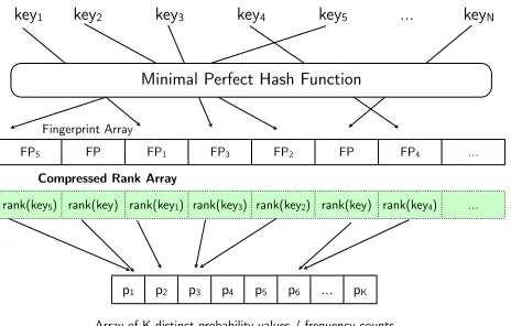
4 Compressed MPHR Approach
Our second approach, called Compressed MPHR, further reduces the size of the model whilst main-taining O(1) time to query the model. Most com-pression techniques work by exploiting the redun-dancy in data. Our fingerprints are unfortunately random sequences of bits, so trying to compress
FP5 FP FP1 FP3 FP2 FP FP4 ...
key1 key2 key3 key4 key5 ... keyN
Minimal Perfect Hash Function
Array of K distinct probability values / frequency counts
p1 p2 p3 p4 p5 p6 ... pK
rank(key5) rank(key) rank(key1) rank(key3) rank(key2) rank(key) rank(key4) ...
Fingerprint Array
[image:6.612.73.300.54.144.2]Compressed Rank Array
Figure 2: Compressed MPHR structure
these is fruitless, but the ranks associated with
n-grams contain much redundancy and so are likely to compress well. We therefore modify our original ar-chitecture to put the ranks and fingerprints into sep-arate arrays, of which the ranks array will be com-pressed, as shown in Figure 2.
Much like the final stage of the CHD minimal perfect hash algorithm we employ a random access compression algorithm of Fredriksson and Nikitin (2007) to reduce the size required by the array of ranks. This method allows compression while re-taining O(1) access to query the model.
The first step in the compression is to encode the ranks array using a dense variable length cod-ing. This coding works by assigning binary codes with different lengths to each number in the rank ar-ray, based on how frequent that number occurs. Let s1, s2, s3, . . . , sKbe the ranks that occur in the rank
array sorted by there frequency. Starting with most
frequent number in the rank array (clearly 1is the
most common frequency count in the data unless it
has been pruned)s1 we assign it the bit code0and
then assigns2the bit code1, we then proceed by
as-signing bit codes of two bits, sos3is assigned00,s4
is assigned01, etc. until all two bit codes are used
up. We then proceed to assign 3 bit codes and so on. All of the values from the rank array are coded in this form and concatenated to form a large bit vector retaining their original ordering. The length in bits
for theith number is thusblog2(i+ 2)cand so the
number of bits required for the whole variable length
coded rank array is: b=PK
i=0f(si)blog2(i+ 2)c.
andKis the total number of distinct ranks. The code
for theith number is the binary representation with
lengthblog2(i+ 2)c of the number obtained using
the formula:
code=i+ 2−2blog2(i+2)c
This variable length coded array is not useful by it-self because we do not know where each number be-gins and ends, so we also store an index array hold this information. We create an additional bit array
Dof the same sizebas the variable length coded
ar-ray that simply contains ones in all positions that a code begins in the rank array and zeros in all other
positions. That is theith rank in the variable length
coded array occurs at position select1(D, i), where
select1 gives the position of the ith one in the
ar-ray. We do not actually store theDarray, but instead
we build a more space efficient structure to answer
select1 queries. Due the distribution ofn-gram
fre-quencies, theDarray is typically dense in
contain-ing a large proportion of ones, so we build arank9sel
dictionary structure (Vigna, 2008) to answer these queries in constant time. We can use this structure
to identify the ith code in our variable length
en-coded rank array by querying for its starting posi-tion, select1(D, i), and compute its length using its
ending position, select1(D, i+ 1)−1. The code and
its length can then be decoded to obtain the original rank:
rank=code+ 2(length in bits)−2
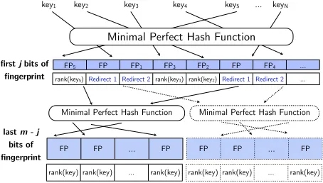
5 Tiered MPHR
In this section we describe an alternative route to ex-tending our basic S-MPHR model to achieve better space efficiency, by using multiple hash stores. The method exploits distributional characteristics of the data, i.e. that lower rank values (those assigned to
values shared by very manyn-grams) are sufficient
for representing the value information of a dispro-portionately large subset of the data. For the Google Web 1T data, for example, we find that the first 256
ranks account for nearly 85% of distinctn-grams, so
if we could store ranks for thesen-grams using only
the 8 bits they require, whilst allowing perhaps 20
bits per n-gram for the remaining 15%, we would
achieve an average of just under 10 bits pern-gram
to store all the rank values.
To achieve this gain, we might partition the
n-gram data into subsets requiring different amounts of space for value storage, and put these subsets in separate MPHRs, e.g. for the example just men-tioned, with two MPHRs having 8 and 20 bit value storage respectively. Partitioning to a larger number
hof MPHRs might further reduce this average cost.
This simple approach has several problems. Firstly,
it potentially requires aseriesof look up steps (i.e.
up toh) to retrieve the value for anyn-gram, with
allhashes needing to be addressed to determine the
unseen status of an unseenn-gram. Secondly,
mul-tiple look ups will produce acompoundingof error
rates, since we have up tohopportunities to falsely
construe an unseenn-gram as seen, or to construe
a seenn-gram as being stored in the wrong MPHR
and so return an incorrect count for it.
FP5 FP FP1 FP3 FP2 FP FP4 ...
key1 key2 key3 key4 key5 ... keyN
Minimal Perfect Hash Function #1
rank(key5) Redirect 1 Redirect 2 rank(key3) rank(key2) Redirect 1 Redirect 2 ...
Minimal Perfect Hash Function #2 Minimal Perfect Hash Function #3
[image:7.612.315.541.301.446.2]rank(key) rank(key) ... rank(key) rank(key) rank(key) ... rank(key)
Figure 3: Tiered minimal perfect hash data structure
We will here explore an alternative approach that
we callTieredMPHR, which avoids this
compound-ing of errors, and which limits the number of looks ups to a maximum of 2, irrespective of how many hashes are used. This approach employs a single
top-levelMPHR which has the full set of n-grams
for its key-set, and stores a fingerprint for each. In addition, space is allocated to store rank values, but with some possible values being reserved to indicate
redirectionto other secondaryhashes where values
can be found. Each secondary hash has a minimal perfect hash function that is computed only for the n-grams whose values it stores. Secondary hashes
donotneed to record fingerprints, as fingerprint
test-ing is done in the top-level hash.
three hashes, with the top-level MPHR having 8-bit storage, and with secondary hashes having 10 and 20 bit storage respectively. Two values of the 8-bit store (e.g. 0 and 1) are reserved to indicate redirection to the specific secondary hashes, with the remaining values (2 . . 255) representing ranks 1 to 254. The 10-bit secondary hash can store 1024 different val-ues, which would then represent ranks 255 to 1278, with all ranks above this being represented in the
20-bit hash. To look up the count for an n-gram,
we begin with the top-level hash, where fingerprint
testing can immediately reject unseenn-grams. For
some seenn-grams, the required rank value is
pro-vided directly by the top-level hash, but for others a redirection value is returned, indicating precisely the secondary hash in which the rank value will be found by simple look up (with no additional finger-print testing). Figure 3 gives a generalized presenta-tion of the structure of tiered MPHRs. Let us repre-sent a configuration for a tiered MPHR as a sequence
of bit values for their value stores, e.g. (8,10,20)
for the example above, or H = (b1, . . . .bh) more
generally (withb1being the top-level MPHR).
The overall memory cost of a particular config-uration depends on distributional characteristics of
the data stored. The top-level MPHR of
config-uration (b1, . . . .bh) stores all n-grams in its
key-set, so its memory cost is calculated as before as
N ×(2.07 +m+b1)(mthe fingerprint size). The
top-level MPHR must reserveh−1values for
redi-rection, and so covers ranks[1. .(2b1−h+ 1)]. The
second MPHR then covers the next2b2 ranks,
start-ing at(2b1−h+ 2), and so on for further secondary
MPHRs. This range of ranks determines the
pro-portion µi of the overalln-gram set that each
sec-ondary MPHRbi stores, and so the memory cost of
each secondary MPHR isN×µi×(2.07 +bi). The
optimal T-MPHR configuration for a given data set is easily determined from distributional information (of the coverage of each rank), by a simple search.
6 Results
In this section, we present some results comparing the performance of our new storage methods to some of the existing methods, regarding the costs of stor-ing LMs, and regardstor-ing the data access speeds that alternative systems allow.
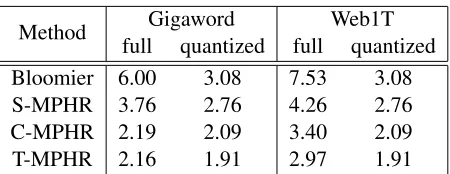
Method Gigaword Web1T
full quantized full quantized
Bloomier 6.00 3.08 7.53 3.08
S-MPHR 3.76 2.76 4.26 2.76
C-MPHR 2.19 2.09 3.40 2.09
T-MPHR 2.16 1.91 2.97 1.91
Table 3: Space usage in bytes/ngram using12-bit finger-prints and storing all 1 to 5 grams
Method Gigaword Web1T
full quantized full quantized
Bloomier 5.38 2.46 6.91 2.46
S-MPHR 3.26 2.26 3.76 2.26
C-MPHR 1.69 1.59 2.90 1.59
[image:8.612.315.540.52.139.2]T-MPHR 1.66 1.41 2.47 1.41
Table 4: Space usage in bytes/n-gram using8-bit finger-prints and storing all 1 to 5 grams
6.1 Comparison of memory costs
To test the effectiveness of our models we built
mod-els storing n-grams and full frequency counts for
both the Gigaword and Google Web1T corpus stor-ing all 1,2,3,4 and 5 grams. These corpora are very large, e.g. the Google Web1T corpus is 24.6GB when gzip compressed and contains over 3.7
bil-lion n-grams, with frequency counts as large as 95
billion, requiring at least 37 bits to be stored. Us-ing the Bloomier algorithm of Talbot and Brants (2008) with 37 bit values and 12 bit fingerprints would require 7.53 bytes/n-gram, so we would need 26.63GB to store a model for the entire corpus.
In comparison, our S-MPHR method requires
only 4.26 bytes per n-gram to store full frequency
count information and stores the entire Web1T
cor-pus in just15.05GBor57%of the space required by
the Bloomier method. This saving is mostly due to the ranking method allowing values to be stored at a
cost of only 20 bits pern-gram. Applying the same
rank array optimization to the Bloomier method sig-nificantly reduces its memory requirement, but S-MPHR still uses only 86% of the space that the
Bloomier approach requires. Using T-MPHR
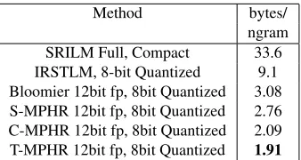
T-Method bytes/ ngram SRILM Full, Compact 33.6 IRSTLM, 8-bit Quantized 9.1 Bloomier 12bit fp, 8bit Quantized 3.08 S-MPHR 12bit fp, 8bit Quantized 2.76 C-MPHR 12bit fp, 8bit Quantized 2.09 T-MPHR 12bit fp, 8bit Quantized 1.91
Table 5: Comparison between approaches for storing all 1 to 5 grams of the Gigaword Corpus
MPHR can store this data in just 8.74GB.
Tables 3, 4 and 5 show results for all methods2on
both corpora, for storing full counts, and for when 8-bit binning quantization of counts is used.
6.2 Access speed comparisons
The three models we present in this paper perform queries in O(1) time and are thus asymptotically optimal, but this does not guarantee they perform well in practice, therefore in this section we
mea-sure query speed on a large set ofn-grams and
com-pare it to that of modern language modeling toolk-its. We build a model of all unigrams and bigrams in the Gigaword corpus (see Table 1) using the C-MPHR method, SRILM (Stolcke, 2002), IRSTLM
(Federico and Cettolo, 2007), and randLM3(Talbot
and Osborne, 2007a) toolkits. RandLM is a mod-ern language modeling toolkit that uses Bloom filter based structures to store large language models and has been integrated so that it can be used as the lan-guage model storage for the Moses statistical ma-chine translation system (Koehn et al., 2007). We
use randLM with the BloomMap (Talbot and
Tal-bot, 2008) storage structure option with 8 bit quan-tized values and an error rate equivalent to using 8 bit fingerprints (as recommended in the Moses doc-umentation). All methods are implemented in C++ and are run on a machine with 2.80GHz Intel Xeon E5462 processor and 64 GB of RAM. In addition we show a comparison to using a modern database, MySQL 5.0, to store the same data. We measure the speed of querying all models for the 55 mil-lion distinct bigrams that occur in the Gigaword,
2
All T-MPHR results are for optimal configurations: Gi-gaword full:(2,3,16), Gigaword quant:(1,8), Web1T full:(8,6,7,8,9,10,13,20), Web1T quant:(1,8).
3http://sourceforge.net/projects/randlm/
Test Time Speed
(hr :min:sec) queries/sec
C-MPHR 00 : 01 : 50 507362
IRSTLM 00 : 02 : 12 422802
SRILM 00 : 01 : 29 627077
randLM 00 : 27 : 28 33865
MySQL 5 29 : 25 : 01 527
Table 6: Look-up speed performance comparison for C-MPHR and several other LM storage methods
these results are shown in Table 6. Unsurprisingly all methods perform significantly faster than using a database as they build models that reside completely in memory. The C-MPHR method tested here is slower than both S-MPHR and T-MPHR models due to the extra operations required for access to the vari-able length encoded array yet still performs similarly to SRILM and IRSTLM and is 14.99 times faster than using randLM.
7 Variable Length Fingerprints
To conclude our presentation of new methods for space-efficient language model storage, we suggest an additional possibility for reducing storage costs, which involves using different sizes of fingerprint
for differentn-grams. Recall that the only errors
al-lowed by our approach are false-positives, i.e. where
an unseenn-gram is falsely construed as being part
of the model and a value returned for it. The idea be-hind using different sizes of fingerprint is that, intu-itively, some possible errors seem worse than others, and in particular, it seems likely to be less damaging
if we falsely construe an unseenn-gram as being a
seenn-gram that has a low count or probability than
as being one with a high count or probability. False positives arise when our perfect hashing
method maps an unseen n-gram to position where
the stored n-gram fingerprint happens to coincide
with that computed for the unseenn-gram. The risk
of this occurring is a simple function of the size of fingerprints. To achieve a scheme that admits a higher risk of less damaging errors, but enforces a lower risk of more damaging errors, we need only
store shorter fingerprints forn-grams in our model
that have low counts or probabilities, and longer
[image:9.612.335.521.53.152.2]idea could be implemented in different ways, e.g. by storing fingerprints of different lengths contigu-ously within a bit array, and constructing a ‘selection structure’ of the kind described in Section 4 to allow us to locate a given fingerprint within the bit array.
FP5 FP FP1 FP3 FP2 FP FP4 ...
key1 key2 key3 key4 key5 ... keyN
Minimal Perfect Hash Function
rank(key5)Redirect 1 Redirect 2 rank(key3) rank(key2)Redirect 1 Redirect 2 ...
Minimal Perfect Hash Function
rank(key) rank(key) ... rank(key)
Minimal Perfect Hash Function
first j bits of fingerprint
FP FP ... FP
last m - j
bits of fingerprint
rank(key) rank(key) ... rank(key)
[image:10.612.318.536.53.192.2]FP FP ... FP
Figure 4: Variable length fingerprint T-MPHR structure using j bit fingerprints for then-grams which are most rare andmbit fingerprints for all others.
We here instead consider an alternative imple-mentation, based on the use of tiered structures. Re-call that for T-MPHR, the top-level MPHR has all n-grams of the model as keys, and stores a fin-gerprint for each, plus a value that may represent
an n-gram’s count or probability, or that may
redi-rect to a second-level hash where that information can be found. Redirection is done for items with higher counts or probabilities, so we can achieve lower error rates for precisely these items by
stor-ing additional fingerprint information for them in
the second-level hash (see Figure 4). For example, we might have a top-level hash with only 4-bit fin-gerprints, but have an additional 8-bits of fingerprint for items also stored in a second-level hash, so there
is quite a high risk (close to 161) of returning a low
count for an unseenn-gram, but a much lower risk
of returning any higher count. Table 7 applies this idea to storing full and quantized counts of the Gi-gaword and Web 1T models, when fingerprints in the top-level MPHR have sizes in the range 1 to 6 bits, with the fingerprint information for items stored in secondary hashes being ‘topped up’ to 12 bits. This approach achieves storage costs of around 1 byte per n-gram or less for the quantized models.
Bits in lowest finger-print
Giga-word Quan-tized
Web1T Quan-tized
Giga-word All
Web1T All
1 0.55 0.55 1.00 1.81
2 0.68 0.68 1.10 1.92
3 0.80 0.80 1.21 2.02
4 0.92 0.92 1.31 2.13
5 1.05 1.04 1.42 2.23
[image:10.612.72.299.150.279.2]6 1.17 1.17 1.52 2.34
Table 7: Bytes per fingerprint for T-MPHR model using 1 to 6 bit fingerprints for rarestn-grams and 12 bit (in total) fingerprints for all othern-grams. (All configurations are as in Footnote 2.)
8 Conclusion
We have presented novel methods of storing large
language models, consisting of billions ofn-grams,
that allow for quantized values or frequency counts to be accessed quickly and which require far less space than all known approaches. We show that it is possible to store all 1 to 5 grams in the Gigaword corpus, with full count information at a cost of just
1.66 bytes pern-gram, or with quantized counts for
just 1.41 bytes pern-gram. We have shown that our
models allown-gram look-up at speeds comparable
to modern language modeling toolkits (which have much greater storage costs), and at a rate approxi-mately 15 times faster than a competitor approach for space-efficient storage.
References
Djamal Belazzougui, Fabiano Botelho, and Martin Diet-zfelbinger. 2009. Hash, displace, and compress. Al-gorithms - ESA 2009, pages 682–693.
Burton H. Bloom. 1970. Space/time trade-offs in hash coding with allowable errors. Commun. ACM, 13(7):422–426.
Thorsten Brants and Alex Franz. 2006. Google Web 1T 5-gram Corpus, version 1. Linguistic Data Con-sortium, Philadelphia, Catalog Number LDC2006T13, September.
Philip Clarkson and Ronald Rosenfeld. 1997. Statis-tical language modeling using the CMU-cambridge toolkit. In Proceedings of ESCA Eurospeech 1997, pages 2707–2710.
Marcello Federico and Nicola Bertoldi. 2006. How many bits are needed to store probabilities for phrase-based translation? InStatMT ’06: Proceedings of the Workshop on Statistical Machine Translation, pages 94–101, Morristown, NJ, USA. Association for Com-putational Linguistics.
Marcello Federico and Mauro Cettolo. 2007. Efficient handling of n-gram language models for statistical ma-chine translation. InStatMT ’07: Proceedings of the Second Workshop on Statistical Machine Translation, pages 88–95, Morristown, NJ, USA. Association for Computational Linguistics.
Edward Fredkin. 1960. Trie memory. Commun. ACM, 3(9):490–499.
Kimmo Fredriksson and Fedor Nikitin. 2007. Simple compression code supporting random access and fast string matching. In Proc. of the 6th International Workshop on Efficient and Experimental Algorithms (WEA’07), pages 203–216.
Ulrich Germann, Eric Joanis, and Samuel Larkin. 2009. Tightly packed tries: How to fit large models into memory, and make them load fast, too. Proceedings of the Workshop on Software Engineering, Testing, and Quality Assurance for Natural Language (SETQA-NLP 2009), pages 31–39.
Joshua Goodman and Jianfeng Gao. 2000. Language model size reduction by pruning and clustering. In Proceedings of ICSLP’00, pages 110–113.
David Graff. 2003. English Gigaword. Linguistic Data Consortium, catalog number LDC2003T05.
Boulos Harb, Ciprian Chelba, Jeffrey Dean, and Sanjay Ghemawat. 2009. Back-off language model compres-sion. InProceedings of Interspeech, pages 352–355. Bo-June Hsu and James Glass. 2008. Iterative language
model estimation:efficient data structure & algorithms. InProceedings of Interspeech, pages 504–511. F. Jelinek, B. Merialdo, S. Roukos, and M. Strauss I.
1990. Self-organized language modeling for speech recognition. InReadings in Speech Recognition, pages 450–506. Morgan Kaufmann.
Philipp Koehn, Hieu Hoang, Alexandra Birch, Chris Callison-Burch, Marcello Federico, Nicola Bertoldi, Brooke Cowan, Wade Shen, Christine Moran, Richard Zens, Chris Dyer, Ondˇrej Bojar, Alexandra Con-stantin, and Evan Herbst. 2007. Moses: open source toolkit for statistical machine translation. InACL ’07: Proceedings of the 45th Annual Meeting of the ACL on Interactive Poster and Demonstration Sessions, pages 177–180, Morristown, NJ, USA. Association for Com-putational Linguistics.
Andreas Stolcke. 1998. Entropy-based pruning of backoff language models. InProceedings of DARPA Broadcast News Transcription and Understanding Workshop, pages 270–274.
Andreas Stolcke. 2002. SRILM - an extensible lan-guage modeling toolkit. In Proceedings of the Inter-national Conference on Spoken Language Processing, volume 2, pages 901–904, Denver.
David Talbot and Thorsten Brants. 2008. Randomized language models via perfect hash functions. Proceed-ings of ACL-08 HLT, pages 505–513.
David Talbot and Miles Osborne. 2007a. Randomised language modelling for statistical machine translation. In Proceedings of ACL 07, pages 512–519, Prague, Czech Republic, June.
David Talbot and Miles Osborne. 2007b. Smoothed bloom filter language models: Tera-scale LMs on the cheap. InProceedings of EMNLP, pages 468–476. David Talbot and John M. Talbot. 2008. Bloom maps.
In 4th Workshop on Analytic Algorithmics and Com-binatorics 2008 (ANALCO’08), pages 203—212, San Francisco, California.
David Talbot. 2009. Succinct approximate counting of skewed data. In IJCAI’09: Proceedings of the 21st international jont conference on Artifical intelligence, pages 1243–1248, San Francisco, CA, USA. Morgan Kaufmann Publishers Inc.
Sebastiano Vigna. 2008. Broadword implementation of rank/select queries. In WEA’08: Proceedings of the 7th international conference on Experimental algo-rithms, pages 154–168, Berlin, Heidelberg. Springer-Verlag.