Attention is not not Explanation

Proceedings of the 2019 Conference on Empirical Methods in Natural Language Processing 11

Attention is not not Explanation

Sarah Wiegreffe⇤

School of Interactive Computing Georgia Institute of Technology

saw@gatech.edu

Yuval Pinter⇤

School of Interactive Computing Georgia Institute of Technology

uvp@gatech.edu

Abstract

Attention mechanisms play a central role in NLP systems, especially within recurrent neu-ral network (RNN) models. Recently, there has been increasing interest in whether or not the intermediate representations offered by these modules may be used to explain the rea-soning for a model’s prediction, and conse-quently reach insights regarding the model’s decision-making process. A recent paper claims that ‘Attention is not Explanation’ (Jain and Wallace, 2019). We challenge many of the assumptions underlying this work, argu-ing that such a claim depends on one’s defi-nition of explanation, and that testing it needs to take into account all elements of the model. We propose four alternative tests to determine when/whether attention can be used as ex-planation: a simple uniform-weights baseline; a variance calibration based on multiple ran-dom seed runs; a diagnostic framework using frozen weights from pretrained models; and an end-to-end adversarial attention training pro-tocol. Each allows for meaningful interpreta-tion of atteninterpreta-tion mechanisms in RNN models. We show that even when reliable adversarial distributions can be found, they don’t perform well on the simple diagnostic, indicating that prior work does not disprove the usefulness of attention mechanisms for explainability.

1 Introduction

Attention mechanisms (Bahdanau et al.,2014) are nowadays ubiquitous in NLP, and their suitabil-ity for providing explanations for model predic-tions is a topic of high interest (Xu et al., 2015; Rockt¨aschel et al.,2015;Mullenbach et al.,2018; Thorne et al., 2019; Serrano and Smith, 2019). If they indeed offer such insights, many applica-tion areas would benefit by better understanding the internals of neural models that use attention

⇤_{Equal contributions.}

as a means for, e.g., model debugging or architec-ture selection. A recent paper (Jain and Wallace, 2019) points to possible pitfalls that may cause re-searchers to misapply attention scores as explana-tions of model behavior, based on a premise that explainable attention distributions should be con-sistentwith other feature-importance measures as well asexclusivegiven a prediction.1 _{Its core}

ar-gument, which we elaborate in §2, is that if al-ternative attention distributions exist that produce similar results to those obtained by the original model, then the original model’s attention scores cannot be reliably used to “faithfully” explain the model’s prediction. Empirically, the authors show that achieving such alternative distributions is easy for a large sample of English-language datasets.

We contend (§2.1) that while Jain and Wal-lace ask an important question, and raise a gen-uine concern regarding potential misuse of atten-tion weights in explaining model decisions on English-language datasets, some key assumptions used in their experimental design leave an implau-sibly large amount of freedom in the setup, ulti-mately leaving practitioners without an applicable way for measuring the utility of attention distribu-tions in specific settings.

We apply a more model-driven approach to this question, beginning (§3.2) with testing atten-tion modules’ contribution to a model by ap-plying a simple baseline where attention weights are frozen to a uniform distribution. We demon-strate that for some datasets, a frozen attention distribution performs just as well as learned at-tention weights, concluding that randomly- or adversarially-perturbed distributions are not

ev-1_{A preliminary version of our theoretical argumentation} was published as a blog post on Medium athttp://bit. ly/2OTzU4r. Following the ensuing online discussion, the authors uploaded a post-conference version of the paper to arXiv(V3) which addresses some of the issues in the post.

the movie was good Prediction Score

Attention Scores

Attention Parameters

LSTM

Embedding

;

MLP

J&W

§3.2 §3.3 §3.4 §4

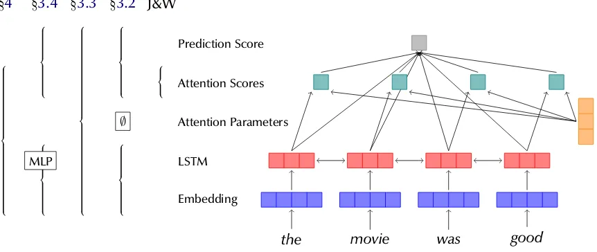
Figure 1: Schematic diagram of a classification LSTM model with attention, including the components manipu-lated or replaced in the experiments performed inJain and Wallace(2019) and in this work (by section).

idence against attention as explanation in these cases. We next (§3.3) examine theexpected vari-ance in attention-produced weights by initializ-ing multiple traininitializ-ing sequences with different ran-dom seeds, allowing a better quantification of how much variance can be expected in trained mod-els. We show that considering this background stochastic variation when comparing adversarial results with a traditional model allows us to better interpret adversarial results. In §3.4, we present a simple yet effectivediagnostic toolwhich tests attention distributions for their usefulness by us-ing them as frozen weights in a non-contextual multi-layered perceptron (MLP) architecture. The favorable performance of LSTM-trained weights provides additional support for the coherence of trained attention scores. This demonstrates a sense in which attention components indeed provide a meaningful model-agnostic interpretation of to-kens in an instance.

In §4, we introduce amodel-consistenttraining protocol for finding adversarial attention weights, correcting some flaws we found in the previous approach. We train a model using a modified loss function which takes into account the distance from an ordinarily-trained base model’s attention scores in order to learn parameters for adversarial attention distributions. We believe these experi-ments are now able to support or refute a claim of faithful explainability, by providing a way for con-vincingly saying by construction that a plausible alternative ‘explanation’ can (or cannot) be con-structed for a given dataset and model architecture. We find that while plausibly adversarial

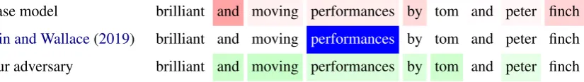
distribu-tions of the consistent kind can indeed be found for the binary classification datasets in question, they are not as extreme as those found in the inconsis-tent manner, as illustrated by an example from the IMDBtask in Figure 2. Furthermore, these

out-puts do not fare well in the diagnostic MLP, call-ing into question the extent to which we can treat them as equally powerful for explainability.

Finally, we provide a theoretical discussion (§5) on the definitions of interpretability and explain-ability, grounding our findings within the accepted definitions of these concepts.

Our four quantitative experiments are illustrated inFigure 1, where each bracket on the left covers the components in a standard RNN-with-attention architecture which we manipulate in each experi-ment. We urge NLP researchers to consider apply-ing the techniques presented here on their mod-els containing attention in order to evaluate its effectiveness at providing explanation. We offer our code for this purpose athttps://github.

com/sarahwie/attention.

2 Attention Might be Explanation

In this section, we briefly describe the experimen-tal design of Jain and Wallace (2019) and look at the results they provide to support their claim that ‘Attention is not explanation’. The authors select eight classification datasets, mostly binary, and two question answering tasks for their experi-ments (detailed in §3.1).

Base model brilliant and moving performances by tom and peter finch Jain and Wallace(2019) brilliant and moving performances by tom and peter finch Our adversary brilliant and moving performances by tom and peter finch

Figure 2: Attention maps for an IMDb instance (all predicted as positive with score> 0.998), showing that in practice it is difficult to learn a distant adversary which is consistent on all instances in the training set.

They find that attention is not strongly correlated with other, well-grounded feature importance met-rics, specifically gradient-based and leave-one-out methods (which in turn correlate well with each other). This experiment evaluates the authors’ claim ofconsistency – that attention-based meth-ods of explainability cannot be valid if they do not correlate well with other metrics. We find the ex-periments in this part of the paper convincing and do not focus our analysis here. We offer our simple MLP diagnostic network (§3.4) as an additional way for determining validity of attention distribu-tions, in a morein vivosetting.

Next, the authors present an adversarial search for alternative attention distributions which mini-mally change model predictions. To this end, they manipulate the attention distributions of trained models (which we will callbasefrom now on) to discern whether alternative distributions exist for which the model outputs near-identical prediction scores. They are able to find such distributions, first by randomly permuting the base attention dis-tributions on the test data during model inference, and later by adversarially searching for maximally different distributions that still produce a predic-tion score within✏of the base distribution. They

use these experimental results as supporting evi-dence for the claim that attention distributions can-not be explainable because they are can-notexclusive. As stated, the lack of comparable change in pre-diction with a change in attention scores is taken as evidence for a lack of “faithful” explainability of the attention mechanism from inputs to output.

Notably, Jain and Wallace detach the attention distribution and output layer of their pretrained network from the parameters that compute them (see Figure 1), treating each attention score as a standalone unit independent of the model. In addi-tion, they compute an independent adversarial dis-tribution for each instance.

2.1 Main Claim

We argue that Jain and Wallace’s counterfactual attention weight experiments do not advance their thesis, for the following reasons:

Attention Distribution is not a Primitive.

From a modeling perspective, detaching the atten-tion scores obtained by parts of the model (i.e. the attention mechanism) degrades the model itself. The base attention weights are not assigned arbi-trarily by the model, but rather computed by an in-tegral component whose parameters were trained alongside the rest of the layers; the way they work depends on each other. Jain and Wallace provide alternative distributions which may result in simi-lar predictions, but in the process they remove the very linkage which motivates the original claim of attention distribution explainability, namely the fact that the model wastrainedto attend to the to-kens it chose. A reliable adversary must take this consideration into account, as our setup in §4does.

Existence does not Entail Exclusivity. On a more theoretical level, we hold that attention scores are used as providing an explanation; not

the explanation. The final layer of an LSTM model may easily produce outputs capable of be-ing aggregated into the same prediction in various ways, however the model still makes the choice of a specific weighting distribution using its trained attention component. This mathematically flexi-ble production capacity is particularly evident in binary classifiers, where prediction is reduced to a single scalar, and an average instance (of e.g. the IMDBdataset) might contain 179 tokens, i.e. 179

scalars to be aggregated. This effect is greatly ex-acerbated when performed independently on each instance.2_{Thus, it is no surprise thatJain and}

Dataset Avg. Length Train Size Test Size (tokens) (neg/pos) (neg/pos) Diabetes 1858 6381/1353 1295/319 Anemia 2188 1847/3251 460/802 IMDb 179 12500/12500 2184/2172

SST 19 3034/3321 863/862

AgNews 36 30000/30000 1900/1900 20News 115 716/710 151/183

Table 1: Dataset statistics.

lace find what they are looking for given this de-gree of freedom.

In summary, due to the per-instance nature of the demonstration and the fact that model parame-ters have not been learned or manipulated directly, Jain and Wallacehavenot shown the existence of an adversarial modelthat produces the claimed adversarial distributions. Thus, we cannot treat these adversarial attentions as equally plausible or faithful explanations for model prediction. Addi-tionally, they haven’t provided a baseline of how much variation is to be expected in learned atten-tion distribuatten-tions, leaving the reader to quesatten-tion just how adversarial the found adversarial distri-butions are.

3 Examining Attention Distributions

In this section, we apply a careful methodological approach for examining the properties of attention distributions and propose alternatives. We begin by identifying the appropriate scope of the mod-els’ performance and variance, followed by imple-menting an empirical diagnostic technique which measures the model-agnostic usefulness of atten-tion weights in capturing the relaatten-tionship between inputs and output.

3.1 Experimental Setup

In order to make our many points in a succinct fashion as well as follow the conclusions drawn by Jain and Wallace, we focus on experimenting with the binary classification subset of their tasks, and on models with an LSTM architecture (Hochreiter and Schmidhuber,1997), the only one the authors make firm conclusions on. Future work may ex-tend our experiments to extractive tasks like ques-tion answering, as well as other attenques-tion-prone tasks, like seq2seq models.

We experiment on the following datasets: Stan-ford Sentiment Treebank (SST) (Socher et al.,

states are typically affected by the input word to a noticeable degree).

Dataset Attention (Base) Uniform Reported Reproduced

Diabetes 0.79 0.775 0.706 Anemia 0.92 0.938 0.899 IMDb 0.88 0.902 0.879

SST 0.81 0.831 0.822

AgNews 0.96 0.964 0.960 20News 0.94 0.942 0.934

Table 2: Classification F1 scores (1-class) on attention models, both as reported by Jain and Wallace and in our reproduction, and on models forced to use uniform attention over hidden states.

2013), IMDB Large Movie Reviews Corpus

(Maas et al., 2011), 20 NEWSGROUPS (hockey

vs. baseball),3 _{the AG NEWS Corpus,}4 _{and two}

prediction tasks from MIMIC-III ICD9 (John-son et al., 2016): DIABETES and ANEMIA. The

tasks are as follows: to predict positive or neg-ative sentiment from sentences (SST) and movie reviews (IMDB), to predict the topic of news

ar-ticles as either baseball (neg.) or hockey (pos.) in 20 NEWSGROUPS and either world (neg.) or

business (pos.) in AG NEWS, to predict whether a

patient is diagnosed with diabetes from their ICU discharge summary, and to predict whether the pa-tient is diagnosed with acute (neg.) or chronic (pos.) anemia (both MIMIC-III ICD9). We use the dataset versions, including train-test split, pro-vided by Jain and Wallace.5 _{All datasets are in}

English.6 _{Data statistics are provided inTable 1.}

We use a single-layer bidirectional LSTM with

tanhactivation, followed by an additive attention

layer (Bahdanau et al.,2014) and softmax predic-tion, which is equivalent to the LSTM setup of Jain and Wallace. We use the same hyperparame-ters found in that work to be effective in training, which we corroborated by reproducing its results to a satisfactory degree (see middle columns of Ta-ble 2). We refer to this architecture as themain setup, where training results in abase model.

FollowingJain and Wallace, all analysis is per-formed on the test set. We report F1 scores on the positive class, and apply the same metrics they use for model comparison, namely Total Variation

3_{http://qwone.com/˜jason/20Newsgroups/} 4_{http://www.di.unipi.it/˜gulli/AG_}

corpus_of_news_articles.html

5_{https://github.com/successar/}

AttentionExplanation

Distance (TVD) for comparing prediction scores

ˆ

yand Jensen-Shannon Divergence (JSD) for

com-paring weighting distributions↵:

TVD(ˆy1,yˆ2) =

1 2

|Y|

X

i=1

|yˆ1i yˆ2i|;

JSD(↵1,↵2) = 1

2KL[↵1k↵] +¯ 1

2KL[↵2k↵]¯,

where↵¯= ↵1+↵2

2 .

3.2 Uniform as the Adversary

First, we test the validity of the classification tasks and datasets by examining whether attention is necessary in the first place. We argue that if at-tention models are not useful compared to very simple baselines, i.e. their parameter capacity is not being used, there is no point in using their out-comes for any type of explanation to begin with. We thus introduce auniformmodel variant, iden-tical to the main setup except that the attention dis-tribution is frozen to uniform weights over the hid-den states.

The results comparing this baseline with the base model are presented inTable 2. If attention was a necessary component for good performance, we would expect a large drop between the two rightmost columns. Somewhat surprisingly, for three of the classification tasks the attention layer appears to offer little to no improvement whatso-ever. We conclude that these datasets, notably AG NEWS and 20 NEWSGROUPS, are not useful test

cases for the debated question: attention is not ex-planation if you don’t need it. We subsequently ig-nore the two News datasets, but keep SST, which we deem borderline.

3.3 Variance within a Model

We now test whether the variances observed by Jain and Wallacebetween trained attention scores and adversarially-obtained ones are unusual. We do this by repeating their analysis on eight mod-els trained from the main setup using different ini-tialization random seeds. The variance introduced in the attention distributions represents a baseline amount of variance that would be considered nor-mal.

The results are plotted in Figure 3 using the same plane as Jain and Wallace’s Figure 8 (with two of these reproduced as (e-f)). Left-heavy vi-olins are interpreted as data classes for which the

compared model produces attention distributions similar to the base model, and so having an adver-sary that manages to ‘pull right’ supports the argu-ment that distributions are easy to manipulate. We see that SST distributions (c, e) are surprisingly ro-bust to random seed change, validating our choice to continue examining this dataset despite its bor-derline F1 score. On the Diabetes dataset, the neg-ative class is already subject to relneg-atively arbitrary distributions from the different random seed set-tings (d), making the highly divergent results from the overly-flexible adversarial setup (f) seem less impressive. Our consistently-adversarial setup in §4will further explore the difficulty of surpassing seed-induced variance between attention distribu-tions.

3.4 Diagnosing Attention Distributions by Guiding Simpler Models

As a more direct examination of models, and as a complementary approach to Jain and Wallace (2019)’s measurement of backward-pass gradient flows through the model for gauging token impor-tance, we introduce a post-hoc training protocol of a non-contextual modelguidedby pre-set weight distributions. The idea is to examine the predic-tion power of attenpredic-tion distribupredic-tions in a ‘clean’ setting, where the trained parts of the model have no access to neighboring tokens of the instance. If pre-trained scores from an attention model per-form well, we take this to mean they are helpful and consistent, fulfilling a certain sense of explain-ability. In addition, this setup serves as an effective diagnostic tool for assessing the utility of adver-sarial attention distributions: if such distributions are truly alternative, they should be equally useful as guides as their base equivalent, and thus per-form comparably.

Our diagnostic model is created by replacing the main setup’s LSTM and attention parameters with a token-level affine hidden layer withtanh

(a) IMDB(seeds) (c) SST (seeds) (e) SST (adversary)

(b) Anemia (seeds) (d) Diabetes (seeds) (f) Diabetes (adversary)

Figure 3: Densities of maximum JS divergences (x-axis) as a function of the max attention (y-axis) in each instance between the base distributions and: (a-d) models initialized on different random seeds; (e-f) models from a per-instance adversarial setup (replication of Figure 8a, 8c resp. inJain and Wallace(2019)). In each max-attention bin, top (blue) is the negative-label instances, bottom (red) positive-label instances.

the movie was good

Prediction Score

Weights (Imposed) Affine

Embedding

Figure 4: Diagram of the setup in §3.4 (except TRAINEDMLP, which learns weight parameters).

MLP to learn its own attention parameters;7 _Base

LSTM, where we take the weights learned by the base LSTM model’s attention layer; and Adver-sary, based on distributions found adversarially using the consistent training algorithm from §4 be-low (where their results will be discussed).

The results are presented in Table 3. The first important result, consistent across datasets, is that using pre-trained LSTM attention weights is bet-ter than letting the MLP learn them on its own, which is in turn better than the unweighted base-line. Comparing with results from §3.2, we see that this setup also outperforms the LSTM trained with uniform attention weights, suggesting that

7_{This is the same asJain and Wallace’saveragesetup.}

Guide weights Diab. Anemia SST IMDb UNIFORM 0.404 0.873 0.812 0.863 TRAINEDMLP 0.699 0.920 0.817 0.888 BASELSTM 0.753 0.931 0.824 0.905

ADVERSARY(4) 0.503 0.932 0.592 0.700

Table 3: F1 scores on the positive class for an MLP model trained on various weighting guides. For AD -VERSARY, we set 0.001.

the attention module is more important than the word-level architecture for these datasets. These findings strengthen the case counter to the claim that attention weights are arbitrary: independent token-level models that have no access to contex-tual information find them useful, indicating that they encode some measure of token importance which is not model-dependent.

4 Training an Adversary

will demonstrate that the extent to which a model-consistent adversary can be found varies across datasets, and that the dramatic reduction in degree of freedom compared to previous work allows for better-informed analysis.

Model. Given the base model Mb, we train a modelMa whose explicit goal is to provide sim-ilar prediction scores for each instance, while dis-tancing its attention distributions from those of Mb. Formally, we train the adversarial model us-ing stochastic gradient updates based on the fol-lowing loss formula (summed over instances in the minibatch):

L(_Ma,_Mb)(i)=TVD(ˆya(i),yˆ(i)b ) KL(↵(i)a k↵(i)b),

whereyˆ(i) and↵(i) denote predictions and atten-tion distribuatten-tions for an instancei, respectively.

is a hyperparameter which we use to control the tradeoff between relaxing the prediction dis-tance requirement (low TVD) in favor of more divergent attention distributions (high JSD), and vice versa. When this interaction is plotted on a two-dimensional axis, the shape of the plot can be interpreted to either support the ‘attention is not explanation’ hypothesis if it is convex (JSD is eas-ily manipulable), or oppose it if it is concave (early increase in JSD comes at a high cost in prediction precision).

Prediction performance. By definition, our loss objective does not directly consider actual prediction performance. The TVD component pushes it towards the same score as the base model, but our setup does not ensure generaliza-tion from train to test. It would thus be interest-ing to inspect the extent of the implicit F1/TVD relationship. We report the highest F1 scores of models whose attention distributions diverge from the base, on average, by at least 0.4 in JSD, as

well as their setting and corresponding compar-ison metrics, in Table 4 (full results available in Appendix B). All F1 scores are on par with the original model results reported inTable 2, indicat-ing the effectiveness of our adversarial models at imitating base model scores on the test sets.

Adversarial weights as guides. We next apply the diagnostic setup introduced in §3.4by training a guided MLP model on the adversarially-trained attention distributions. The results, reported in the bottom line of Table 3, show that despite

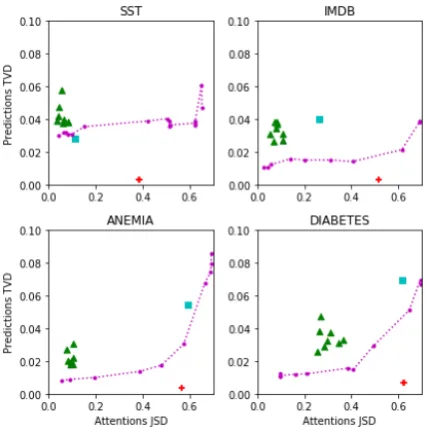
Figure 5: Averaged per-instance test set JSD and TVD from base model for each model variant. JSD is bounded at ⇠ 0.693. N: random seed; ⌅: uniform

weights; dotted line: our adversarial setup as is var-ied;+: adversarial setup fromJain and Wallace(2019).

Dataset F1 (") TVD (#) JSD (") Diabetes 2e-4 0.775 0.015 0.409 Anemia 5e-4 0.942 0.017 0.481 SST 5.25e-4 0.823 0.036 0.514 IMDb 8e-4 0.906 0.014 0.405

Table 4: Best-performing adversarial models with instance-average JSD>0.4.

their local decision-imitation abilities, they are usually completely incapable of providing a non-contextual framework with useful guides.8 _We

of-fer these results as evidence that adversarial dis-tributions, even those obtained consistently for a dataset, deprive the underlying model from some form of understanding it gained over the data, one that it was able to leverage by tuning the attention mechanism towards preferring ‘useful’ tokens.

TVD/JSD tradeoff. In Figure 5 we present the levels of prediction variance (TVD) allowed

by models achieving increased attention distance (JSD) on all four datasets. The convex shape of most curves does lend support to the claim that attention scores are easily manipulable; however the extent of this effect emerging from Jain and Wallace’s per-instance setup is a considerable ex-aggeration, as seen by its position (+) well below the curve of our parameterized model set. Again, the SST dataset emerges as an outlier: not only can JSD be increased practically arbitrarily with-out incurring prediction variance cost, the uniform baseline (⌅) comes up under the curve, i.e. with a better adversarial score. We again include ran-dom seed initializations (N) in order to quantify a baseline amount of variance.

TVD/JSD plots broken down by prediction class are available inAppendix C. In future work, we intend to inspect the potential of multiple ad-versarial attention models existing side-by-side, all distant enough from each other.

Concrete Example. Table 2 illustrates the dif-ference between inconsistently-achieved adversar-ial heatmaps and consistently trained ones. De-spite both adversaries approximating the desired prediction score to very high degree, the heatmaps show thatJain and Wallace’s model has distributed all of the attention weight to an ad-hoc token, whereas our trained model could only distance it-self from the base model distribution by so much, keeping multiple tokens in the>0.1score range.

5 Defining Explanation

The umbrella term of “Explainable AI” encom-passes at least three distinct notions:transparency,

explainability, andinterpretability. Lipton(2016) categorizes transparency, or overall human under-standing of a model, and post-hoc explainability as two competing notions under the umbrella of in-terpretability. The relevant sense of transparency, as defined by Lipton(2016) (§3.1.2), pertains to the way in which a specific portion of a model corresponds to a human-understandable construct (which Doshi-Velez and Kim (2017) refer to as a “cognitive chunk”). Under this definition, it should appear sensible of the NLP community to treat attention scores as a vehicle of (partial) trans-parency. Attention mechanisms do provide a look into the inner workings of a model, as they pro-duce an easily-understandable weighting of hid-den states.

Rudin(2018) defines explainability as simply a plausible (but not necessarily faithful) reconstruc-tion of the decision-making process, and Riedl (2019) classifies explainable rationales as valuable in that they mimic what we as humans do when we rationalize past actions: we invent a story that plausibly justifies our actions, even if it is not an entirely accurate reconstruction of the neural pro-cesses that produced our behavior at the time. Dis-tinguishing between interpretability and explain-ability as two separate notions, Rudin (2018) ar-gues that interpretability is more desirable but more difficult to achieve than explainability, be-cause it requires presenting humans with a big-picture understanding of the correlative relation-ship between inputs and outputs (citing the exam-ple of linear regression coefficients). Doshi-Velez and Kim (2017) break down interpretability into further subcategories, depending on the amount of human involvement and the difficulty of the task.

In prior work,Lei et al.(2016) train a model to simultaneously generate rationales and predictions from input text, using gold-label rationales to eval-uate their model. Generally, many accept the no-tion of extractive methods such asLei et al.(2016), in which explanations come directly from the in-put itself (as in attention), as plausible. Works such asMullenbach et al.(2018) andEhsan et al. (2019) use human evaluation to evaluate explana-tions; the former based on attention scores over the input, and the latter based on systems with addi-tional raaddi-tionale-generation capability. The authors show that rationales generated in a post-hoc man-ner increase user trust in a system.

or meaningless, and under this definition the exis-tence of multiple different explanations is not nec-essarily indicative of the quality of a single one.

Jain and Wallace define attention and explana-tion as measuring the “responsibility” each input token has on a prediction. This aligns more closely with the more rigorous (Lipton,2016, §3.1.1) def-inition of transparency, or Rudin (2018)’s defini-tion of interpretability: human understanding of the model as a whole rather than of its respective parts. The ultimate question posed so far as ‘is at-tention explanation?’ seems to be: do high atten-tion weights on certain elements in the input lead the model to make its prediction? This question is ultimately left largely unanswered by prior work, as we address in previous sections. However, un-der the given definition of transparency, the au-thors’ exclusivity requisite is well-defined and we find value in their counterfactual framework as a concept – if a model is capable of producing mul-tiple sets of diverse attention weights for the same prediction, then the relationship between inputs and outputs used to make predictions is not under-stood by attention analysis. This provides us with the motivation to implement the adversarial setup coherently and to derive and present conclusions from it. To this end, we additionally provide our §3.4 model to test the relationship between input tokens and output.

In the terminology of Doshi-Velez and Kim (2017), our proposed methods provide a

functionally-grounded evaluation of attention as explanation, i.e. an analysis conducted on proxy tasks without human evaluation. We believe the proxies we have provided can be used to test the validity of attention as a form of explanation from the ground-up, based on the type of explanation one is looking for.

6 Attention is All you Need it to Be

Whether or not attention is explanation depends on the definition of explainability one is looking for: plausible or faithful explanations (or both). We believe that prior work focused on providing plausible rationales is not invalidated byJain and Wallace’s or our results. However, we have con-firmed that adversarial distributions can be found for LSTM models in some classification tasks, as originally hypothesized byJain and Wallace. This should provide pause to researchers who are look-ing to attention distributions for one true, faithful

interpretation of the link their model has estab-lished between inputs and outputs. At the same time, we have provided a suite of experiments that researchers can make use of in order to make in-formed decisions about the quality of their mod-els’ attention mechanisms when used as explana-tion for model predicexplana-tions.

We’ve shown that alternative attention distribu-tions found via adversarial training methods per-form poorly relative to traditional attention mech-anisms when used in our diagnostic MLP model. These results indicate that trained attention mech-anisms in RNNs on our datasets do in fact learn something meaningful about the relationship be-tween tokens and prediction which cannot be eas-ily ‘hacked’ adversarially.

We view the conditions under which adversarial distributions can actually be found in practice to be an important direction for future work. Additional future directions for this line of work include ap-plication on other tasks such as sequence modeling and multi-document analysis (NLI, QA); exten-sion to languages other than English; and adding a human evaluation for examining the level of agree-ment with our measures. We also believe our work can provide value to theoretical analysis of atten-tion models, motivating development of analytical methods to estimate the usefulness of attention as an explanation based on dataset and model prop-erties.

Acknowledgments

We thank Yoav Goldberg for preliminary com-ments on the idea behind the original Medium post. We thank the online community who par-ticipated in the discussion following the post, and particularly Sarthak Jain and Byron Wallace for their active engagement, as well as for the high-quality code they released which allowed fast re-production and modification of their experiments. We thank Erik Wijmans for early feedback. We thank the members of the Computational Linguis-tics group at Georgia Tech for discussions and comments, particularly Jacob Eisenstein and Mu-rali Raghu Babu. We thank the anonymous re-viewers for many useful comments.

YP is a Bloomberg Data Science PhD Fellow.

References

learning to align and translate. arXiv preprint arXiv:1409.0473.

Finale Doshi-Velez and Been Kim. 2017. Towards a rigorous science of interpretable machine learning.

arXiv preprint arXiv:1702.08608.

Upol Ehsan, Pradyumna Tambwekar, Larry Chan, Brent Harrison, and Mark O Riedl. 2019. Auto-mated rationale generation: a technique for explain-able ai and its effects on human perceptions. In Pro-ceedings of the 24th International Conference on In-telligent User Interfaces, pages 263–274. ACM. Sepp Hochreiter and J¨urgen Schmidhuber. 1997.

Long short-term memory. Neural computation, 9(8):1735–1780.

Sarthak Jain and Byron C. Wallace. 2019. Attention is not Explanation. In Proceedings of the 2019 Con-ference of the North American Chapter of the Asso-ciation for Computational Linguistics: Human Lan-guage Technologies, Volume 1 (Long Papers), Min-neapolis, Minnesota. Association for Computational Linguistics.

Alistair EW Johnson, Tom J Pollard, Lu Shen, H Lehman Li-wei, Mengling Feng, Moham-mad Ghassemi, Benjamin Moody, Peter Szolovits, Leo Anthony Celi, and Roger G Mark. 2016. Mimic-iii, a freely accessible critical care database.

Scientific data, 3:160035.

Tao Lei, Regina Barzilay, and Tommi Jaakkola. 2016. Rationalizing neural predictions. InProceedings of the 2016 Conference on Empirical Methods in Nat-ural Language Processing, pages 107–117, Austin, Texas. Association for Computational Linguistics. Zachary C Lipton. 2016. The mythos of model

inter-pretability.arXiv preprint arXiv:1606.03490. Andrew L Maas, Raymond E Daly, Peter T Pham, Dan

Huang, Andrew Y Ng, and Christopher Potts. 2011. Learning word vectors for sentiment analysis. In

Proceedings of the 49th annual meeting of the as-sociation for computational linguistics: Human lan-guage technologies-volume 1, pages 142–150. Asso-ciation for Computational Linguistics.

James Mullenbach, Sarah Wiegreffe, Jon Duke, Ji-meng Sun, and Jacob Eisenstein. 2018. Explain-able prediction of medical codes from clinical text. InProceedings of the 2018 Conference of the North American Chapter of the Association for Computa-tional Linguistics: Human Language Technologies, Volume 1 (Long Papers), pages 1101–1111, New Orleans, Louisiana. Association for Computational Linguistics.

Azadeh Nikfarjam, Abeed Sarker, Karen O’connor, Rachel Ginn, and Graciela Gonzalez. 2015. Phar-macovigilance from social media: mining adverse drug reaction mentions using sequence labeling with word embedding cluster features. Journal of the American Medical Informatics Association, 22(3):671–681.

Mark O Riedl. 2019. Human-centered artificial intelli-gence and machine learning. Human Behavior and Emerging Technologies, 1(1):33–36.

Tim Rockt¨aschel, Edward Grefenstette, Karl Moritz Hermann, Tom´aˇs Koˇcisk`y, and Phil Blunsom. 2015. Reasoning about entailment with neural attention.

arXiv preprint arXiv:1509.06664.

Andrew Slavin Ross, Michael C Hughes, and Finale Doshi-Velez. 2017. Right for the right reasons: training differentiable models by constraining their explanations. In Proceedings of the 26th Interna-tional Joint Conference on Artificial Intelligence, pages 2662–2670. AAAI Press.

Cynthia Rudin. 2018. Please stop explaining black box models for high stakes decisions. arXiv preprint arXiv:1811.10154.

Sofia Serrano and Noah A. Smith. 2019. Is attention interpretable? In Proceedings of the 57th Annual Meeting of the Association for Computational Lin-guistics, pages 2931–2951, Florence, Italy. Associa-tion for ComputaAssocia-tional Linguistics.

Richard Socher, Alex Perelygin, Jean Wu, Jason Chuang, Christopher D Manning, Andrew Ng, and Christopher Potts. 2013. Recursive deep models for semantic compositionality over a sentiment tree-bank. In Proceedings of the 2013 conference on empirical methods in natural language processing, pages 1631–1642.

James Thorne, Andreas Vlachos, Christos Christodoulopoulos, and Arpit Mittal. 2019. Generating token-level explanations for natural language inference. In Proceedings of the 2019 Conference of the North American Chapter of the Association for Computational Linguistics: Human Language Technologies, Volume 1 (Long and Short Papers), pages 963–969, Minneapolis, Minnesota. Association for Computational Linguistics.